8. Open Rails Physics

Open Rails physics is in an advanced stage of development. The physics structure is divided into logical classes; more generic classes are parent classes, more specialized classes inherit properties and methods of their parent class. Therefore, the description for train cars physics is also valid for locomotives (because a locomotive is a special case of a train car). All parameters are defined within the .wag or .eng file. The definition is based on MSTS file format and some additional ORTS based parameters. To avoid possible conflicts in MSTS, the ORTS prefix is added to every OpenRails specific parameter (such as ORTSMaxTractiveForceCurves).

The .wag or .eng file may be placed as in MSTS in the TRAINS\TRAINSET\TrainCar\ folder (where TrainCar is the name of the train car folder). If OR-specific parameters are used, or if different .wag or .eng files are used for MSTS and OR, the preferred solution is to place the OR-specific .wag or .eng file in a created folder TRAINS\TRAINSET\TrainCar\OpenRails\ (see here for more).

8.1. Train Cars (WAG, or Wagon Part of ENG file)

The behavior of a train car is mainly defined by a resistance / resistive force (a force needed to pull a car). Train car physics also includes coupler slack and braking. In the description below, the Wagon section of the WAG / ENG file is discussed.

8.1.1. Resistive Forces

Open Rails physics calculates resistance based on real world physics: gravity, mass, rolling resistance and optionally curve resistance. This is calculated individually for each car in the train. The program calculates rolling resistance, or friction, based on the Friction parameters in the Wagon section of .wag/.eng file. Open Rails identifies whether the .wag file uses the FCalc utility or other friction data. If FCalc was used to determine the Friction variables within the .wag file, Open Rails compares that data to the Open Rails Davis equations to identify the closest match with the Open Rails Davis equation. If no-FCalc Friction parameters are used in the .wag file, Open Rails ignores those values, substituting its actual Davis equation values for the train car.

A basic (simplified) Davis formula is used in the following form:

F_res = ORTSDavis_A + speedMpS * (ORTSDavis_B + ORTSDavis_C * speedMpS²)

Where F_res is the friction force of the car. The rolling resistance can be defined either by FCalc or ORTSDavis_A, _B and _C components. If one of the ORTSDavis components is zero, FCalc is used. Therefore, e.g. if the data doesn’t contain the B part of the Davis formula, a very small number should be used instead of zero.

When a car is pulled from steady state, an additional force is needed due to higher bearing forces. The situation is simplified by using a different calculation at low speed (5 mph and lower). Empirical static friction forces are used for different classes of mass (under 10 tons, 10 to 100 tons and above 100 tons). In addition, if weather conditions are poor (snowing is set), the static friction is increased.

When running on a curve and if the Curve dependent resistance option is enabled, additional resistance is calculated, based on the curve radius, rigid wheel base, track gauge and super elevation. The curve resistance has its lowest value at the curve’s optimal speed. Running at higher or lower speed causes higher curve resistance. The worst situation is starting a train from zero speed. The track gauge value can be set by ORTSTrackGauge parameter, otherwise 1435 mm is used. The rigid wheel base can be also set by ORTSRigidWheelBase, otherwise the value is estimated. Further details are discussed later.

When running on a slope (uphill or downhill), additional resistance is calculated based on the car mass taking into account the elevation of the car itself. Interaction with the car vibration feature is a known issue (if the car vibrates the resistance value oscillate).

8.1.2. Coupler Slack

Slack action for couplers is introduced and calculated the same way as in MSTS.

8.1.3. Adhesion of Locomotives – Settings Within the Wagon Section of ENG files

MSTS calculates the adhesion parameters based on a very strange set of parameters filled with an even stranger range of values. Since ORTS is not able to mimic the MSTS calculation, a standard method based on the adhesion theory is used with some known issues in use with MSTS content.

MSTS Adheasion (sic!) parameters are not used in ORTS. Instead, a new set of parameters is used, which must be inserted within the Wagon section of the .ENG file:

ORTSAdhesion (
    ORTSCurtius_Kniffler (A B C D )
)

The A, B and C values are coefficients of a standard form of various empirical formulas, e.g. Curtius-Kniffler or Kother. The D parameter is used in the advanced adhesion model described later.

From A, B and C a coefficient CK is computed, and the adhesion force limit is then calculated by multiplication of CK by the car mass and the acceleration of gravity (9.81), as better explained later.

The adhesion limit is only considered in the adhesion model of locomotives.

The adhesion model is calculated in two possible ways. The first one – the simple adhesion model – is based on a very simple threshold condition and works similarly to the MSTS adhesion model. The second one – the advanced adhesion model – is a dynamic model simulating the real world conditions on a wheel-to-rail contact and will be described later. The advanced adhesion model uses some additional parameters such as:

ORTSAdhesion (
    ORTSSlipWarningThreshold ( T )
)

where T is the wheelslip percentage considered as a warning value to be displayed to the driver; and:

ORTSAdhesion(
    Wheelset (
        Axle (
            ORTSInertia (
                Inertia
            )
        )
    )
)

where Inertia is the model inertia in kg.m2 and can be set to adjust the advanced adhesion model dynamics. The value considers the inertia of all the axles and traction drives. If not set, the value is estimated from the locomotive mass and maximal power.

The first model – simple adhesion model – is a simple tractive force condition-based computation. If the tractive force reaches its actual maximum, the wheel slip is indicated in HUD view and the tractive force falls to 10% of the previous value. By reducing the throttle setting adherence is regained. This is called the simple adhesion model.

The second adhesion model (advanced adhesion model) is based on a simplified dynamic adhesion theory. Very briefly, there is always some speed difference between the wheel speed of the locomotive and the longitudinal train speed when the tractive force is different from zero. This difference is called wheel slip / wheel creep. The adhesion status is indicated in the HUD Force Information view by the Wheel Slip parameter and as a warning in the general area of the HUD view. For simplicity, only one axle model is computed (and animated). A tilting feature and the independent axle adhesion model will be introduced in the future.

The heart of the model is the slip characteristics (picture below).

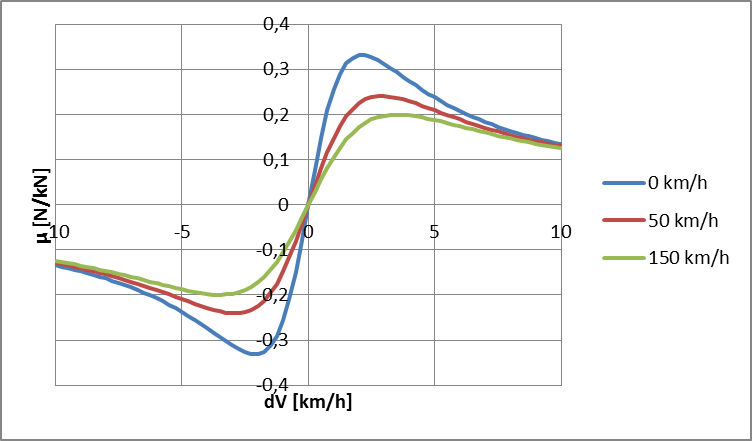
The wheel creep describes the stable area of the characteristics and is used in the most of the operation time. When the tractive force reaches the actual maximum of the slip characteristics, force transition falls down and more power is used to speed up the wheels, so called wheel slip.

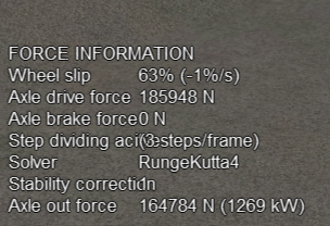
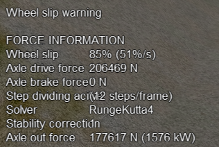
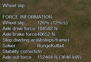
To avoid the loss of the tractive force, use the throttle in combination with sanding to return to the stable area (wheel creep area). A possible sequence of the wheel slip development is shown on the pictures below. The Wheel slip value is displayed as a value relative to the best adhesion conditions for actual speed and weather. The value of 63% means very good force transition. For values higher than ( ORTSadhesion ( ORTSSlipWarningThreshold ) ) or 70% by default, the Wheel slip warning is displayed, but the force transition is still very good. This indication should warn you to use the throttle very carefully. Exceeding 100%, the Wheel slip message is displayed and the wheels are starting to speed up, which can be seen on the speedometer or in external view 2. To reduce the wheel slip, use throttle down, sanding or the locomotive brake.

The actual maximum of the tractive force is based on the Curtius-Kniffler adhesion theory and can be adjusted by the aforementioned ORTSCurtius_Kniffler ( A B C D ) parameters, where A, B, C are coefficients of Curtius-Kniffler, Kother or similar formula. By default, Curtius-Kniffler is used.

\[F_{adhMAX} = W\cdot m\left[\mathrm{kg}\right]\cdot 9.81\left[\mathrm{\frac{m}{s^2}}\right]\cdot\left( \frac{A}{B + v\left[\mathrm{\frac{km}{h}}\right]} + C\right)\]

Where W is the weather coefficient. This means that the maximum is related to the speed of the train, or to the weather conditions.

The D parameter is used in an advanced adhesion model and should always be 0.7.

There are some additional parameters in the Force Information HUD view. The axle/wheel is driven by the Axle drive force and braked by the Axle brake force. The Axle out force is the output force of the adhesion model (used to pull the train). To compute the model correctly the FPS rate needs to be divided by a Solver dividing value in a range from 1 to 50. By default, the Runge-Kutta4 solver is used to obtain the best results. When the Solver dividing value is higher than 40, in order to reduce CPU load the Euler-modified solver is used instead.

In some cases when the CPU load is high, the time step for the computation may become very high and the simulation may start to oscillate (the Wheel slip rate of change (in the brackets) becomes very high). There is a stability correction feature that modifies the dynamics of the adhesion characteristics. Higher instability can cause a huge wheel slip. You can use the DebugResetWheelSlip (<Ctrl+X> keys by default) command to reset the adhesion model. If you experience such behavior most of time, use the basic adhesion model instead by pressing DebugToggleAdvancedAdhesion ( <Ctrl+Alt+X> keys by default).

Another option is to use a Moving average filter available in the Simulation Options. The higher the value, the more stable the simulation will be. However, the higher value causes slower dynamic response. The recommended range is between 10 and 50.

To match some of the real world features, the Wheel slip event can cause automatic zero throttle setting. Use the Engine (ORTS (ORTSWheelSlipCausesThrottleDown)) Boolean value of the ENG file.

8.2. Engine – Classes of Motive Power

Open Rails software provides for different classes of engines: diesel, electric, steam and default. If needed, additional classes can be created with unique performance characteristics.

8.2.1. Diesel Locomotives in General

The diesel locomotive model in ORTS simulates the behavior of two basic types of diesel engine driven locomotives– diesel-electric and diesel-mechanical. The diesel engine model is the same for both types, but acts differently because of the different type of load. Basic controls (direction, throttle, dynamic brake, air brakes) are common across all classes of engines. Diesel engines can be started or stopped by pressing the START/STOP key (<Shift+Y> in English keyboards). The starting and stopping sequence is driven by a starter logic, which can be customized, or is estimated by the engine parameters.

8.2.1.1. Starting the Diesel Engine

To start the engine, simply press the START/STOP key once. The direction controller must be in the neutral position (otherwise, a warning message pops up). The engine RPM (revolutions per minute) will increase according to its speed curve parameters (described later). When the RPM reaches 90% of StartingRPM (67% of IdleRPM by default), the fuel starts to flow and the exhaust emission starts as well. RPM continues to increase up to StartingConfirmationRPM (110% of IdleRPM by default) and the demanded RPM is set to idle. The engine is now started and ready to operate.

8.2.1.2. Stopping the Diesel Engine

To stop the engine, press the START/STOP key once. The direction controller must be in the neutral position (otherwise, a warning message pops up). The fuel flow is cut off and the RPM will start to decrease according to its speed curve parameters. The engine is considered as fully stopped when RPM is zero. The engine can be restarted even while it is stopping (RPM is not zero).

8.2.1.3. Starting or Stopping Helper Diesel Engines

By pressing the Diesel helper START/STOP key (<Ctrl+Y> on English keyboards), the diesel engines of helper locomotives can be started or stopped. Also consider disconnecting the unit from the multiple-unit (MU) signals instead of stopping the engine (see here, Toggle MU connection).

It is also possible to operate a locomotive with the own engine off and the helper’s engine on.

8.2.1.4. ORTS Specific Diesel Engine Definition

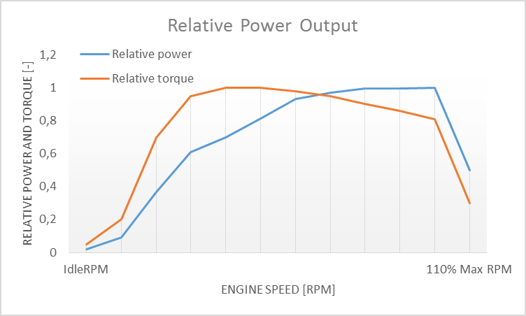
If no ORTS specific definition is found, a single diesel engine definition is created based on the MSTS settings. Since MSTS introduces a model without any data crosscheck, the behavior of MSTS and ORTS diesel locomotives can be very different. In MSTS, MaxPower is not considered in the same way and you can get much better performance than expected. In ORTS, diesel engines cannot be overloaded.

No matter which engine definition is used, the diesel engine is defined by its load characteristics (maximum output power vs. speed) for optimal fuel flow and/or mechanical characteristics (output torque vs. speed) for maximum fuel flow. The model computes output power / torque according to these characteristics and the throttle settings. If the characteristics are not defined (as they are in the example below), they are calculated based on the MSTS data and common normalized characteristics.

In many cases the throttle vs. speed curve is customized because power vs. speed is not linear. A default linear throttle vs. speed characteristics is built in to avoid engine overloading at lower throttle settings. Nevertheless, it is recommended to adjust the table below to get more realistic behavior.

In ORTS, single or multiple engines can be set for one locomotive. In case there is more than one engine, other engines act like helper engines (start/stop control for helpers is <Ctrl+Y> by default). The power of each active engine is added to the locomotive power. The number of such diesel engines is not limited.

If the ORTS specific definition is used, each parameter is tracked and if one is missing (except in the case of those marked with Optional), the simulation falls back to use MSTS parameters.

Engine( ... ORTSDieselEngines ( 2 Diesel ( IdleRPM ( 510 ) MaxRPM ( 1250 ) StartingRPM ( 400 ) StartingConfirmRPM ( 570 ) ChangeUpRPMpS ( 50 ) ChangeDownRPMpS ( 20 ) RateOfChangeUpRPMpSS ( 5 ) RateOfChangeDownRPMpSS ( 5 ) MaximalPower ( 300kW ) IdleExhaust ( 5 ) MaxExhaust ( 50 ) ExhaustDynamics ( 10 ) ExhaustDynamicsDown (10) ExhaustColor ( 00 fe ) ExhaustTransientColor( 00 00 00 00) DieselPowerTab ( 0 0 510 2000 520 5000 600 2000 800 70000 1000 100000 1100 200000 1200 280000 1250 300000 ) DieselConsumptionTab ( 0 0 510 10 1250 245 ) ThrottleRPMTab ( 0 510 5 520 10 600 20 700 50 1000 75 1200 100 1250 ) DieselTorqueTab ( 0 0 510 25000 1250 200000 ) MinOilPressure ( 40 ) MaxOilPressure ( 90 ) MaxTemperature ( 120 ) Cooling ( 3 ) TempTimeConstant ( 720 ) OptTemperature ( 90 ) IdleTemperature ( 70 ) ) Diesel ( ... )

Engine section in eng file Number of engines Idle RPM Maximal RPM Starting RPM Starting confirmation RPM Increasing change rate RPM/s Decreasing change rate RPM/s Jerk of ChangeUpRPMpS RPM/s^2 Jerk of ChangeDownRPMpS RPM/s^2 Maximal output power Num of exhaust particles at IdleRPM Num of exhaust particles at MaxRPM Exhaust particle mult. at transient Mult. for down transient (Optional) Exhaust color at steady state Exhaust color at RPM changing Diesel engine power table RPM Power in Watts Diesel fuel consumption table RPM Vs consumption l/h/rpm Eengine RPM vs. throttle table Throttle % Demanded RPM Diesel engine RPM vs. torque table RPM Force in Newtons Min oil pressure PSI Max oil pressure PSI Maximal temperature Celsius Cooling 0=No cooling, 1=Mechanical, 2= Hysteresis, 3=Proportional Rate of temperature change Normal temperature Celsius Idle temperature Celsius The same as above, or different

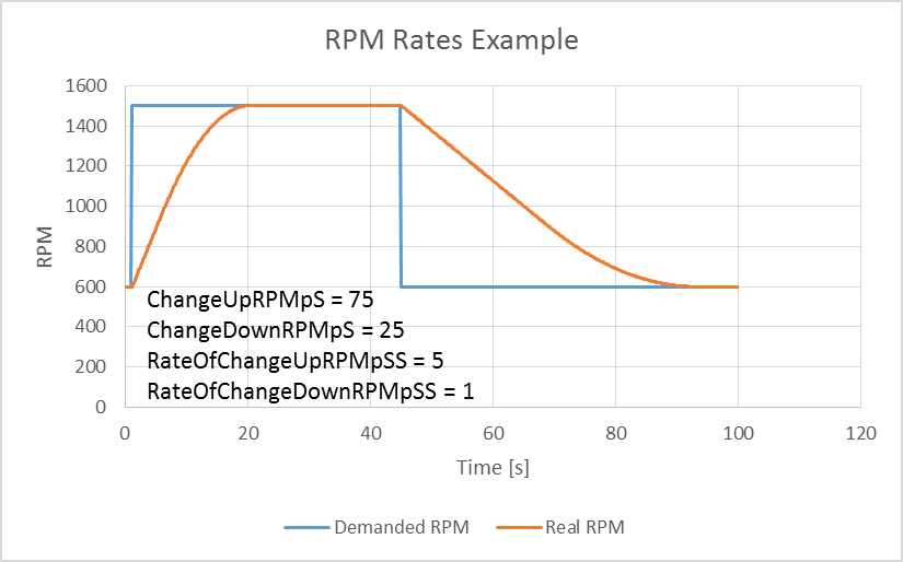
8.2.1.5. Diesel Engine Speed Behavior

The engine speed is calculated based on the RPM rate of change and its rate of change. The usual setting and the corresponding result is shown below. ChangeUpRPMpS means the slope of RPM, RateOfChangeUpRPMpSS means how fast the RPM approaches the demanded RPM.

8.2.1.6. Fuel Consumption

Following the MSTS model, ORTS computes the diesel engine fuel consumption based on .eng file parameters. The fuel flow and level are indicated by the HUD view. Final fuel consumption is adjusted according to the current diesel power output (load).

8.2.1.7. Diesel Exhaust

The diesel engine exhaust feature can be modified as needed. The main idea of this feature is based on the general combustion engine exhaust. When operating in a steady state, the color of the exhaust is given by the new ENG parameter engine (ORTS (Diesel (ExhaustColor))).

The amount of particles emitted is given by a linear interpolation of the values of engine(ORTS (Diesel (IdleExhaust))) and engine(ORTS (Diesel (MaxExhaust))) in the range from 1 to 50. In a transient state, the amount of the fuel increases but the combustion is not optimal. Thus, the quantity of particles is temporarily higher: e.g. multiplied by the value of

engine(ORTS (Diesel (ExhaustDynamics))) and displayed with the color given by engine(ORTS(Diesel(ExhaustTransientColor))).

The format of the color value is (aarrggbb) where:

• aa = intensity of light;
• rr = red color component;
• gg = green color component;
• bb = blue color component;

and each component is in HEX number format (00 to ff).

8.2.1.8. Cooling System

ORTS introduces a simple cooling and oil system within the diesel engine model. The engine temperature is based on the output power and the cooling system output. A maximum value of 100°C can be reached with no impact on performance. It is just an indicator, but the impact on the engine’s performance will be implemented later. The oil pressure feature is simplified and the value is proportional to the RPM. There will be further improvements of the system later.

8.2.2. Diesel-Electric Locomotives

Diesel-electric locomotives are driven by electric traction motors supplied by a diesel-generator set. The gen-set is the only power source available, thus the diesel engine power also supplies auxiliaries and other loads. Therefore, the output power will always be lower than the diesel engine rated power.

In ORTS, the diesel-electric locomotive can use ORTSTractionCharacteristics or tables of ORTSMaxTractiveForceCurves to provide a better approximation to real world performance. If a table is not used, the tractive force is limited by MaxForce, MaxPower and MaxVelocity. The throttle setting is passed to the ThrottleRPMTab, where the RPM demand is selected. The output force increases with the Throttle setting, but the power follows maximal output power available (RPM dependent).

8.2.3. Diesel-Hydraulic Locomotives

Diesel-hydraulic locomotives are not implemented in ORTS. However, by using either ORTSTractionCharacteristics or ORTSMaxTractiveForceCurves tables, the desired performance can be achieved, when no gearbox is in use and the DieselEngineType is electric.

8.2.4. Diesel-Mechanical Locomotives

ORTS features a mechanical gearbox feature that mimics MSTS behavior, including automatic or manual shifting. Some features not well described in MSTS are not yet implemented, such as GearBoxBackLoadForce, GearBoxCoastingForce and GearBoxEngineBraking.

Output performance is very different compared with MSTS. The output force is computed using the diesel engine torque characteristics to get results that are more precise.

8.3. Electric Locomotives

At the present time, diesel and electric locomotive physics calculations use the default engine physics. Default engine physics simply uses the MaxPower and MaxForce parameters to determine the pulling power of the engine, modified by the Reverser and Throttle positions. The locomotive physics can be replaced by traction characteristics (speed in mps vs. force in Newtons) as described below.

Some OR-specific parameters are available in order to improve the realism of the electric system.

8.3.1. Pantographs

The pantographs of all locomotives in a consist are triggered by Control Pantograph First and Control Pantograph Second commands ( <P> and <Shift+P> by default ). The status of the pantographs is indicated by the Pantographs value in the HUD view.

Since the simulator does not know whether the pantograph in the 3D model is up or down, you can set some additional parameters in order to add a delay between the time when the command to raise the pantograph is given and when the pantograph is actually up.

In order to do this, you can write in the Wagon section of your .eng file or .wag file (since the pantograph may be on a wagon) this optional structure:

ORTSPantographs(
    Pantograph(         << This is going to be your first pantograph.
        Delay( 5s )     << Example : a delay of 5 seconds
    )
    Pantograph(
        ... parameters for the second pantograph ...
    )
)

Other parameters will be added to this structure later, such as power limitations or speed restrictions.

8.3.2. Circuit breaker

The circuit breaker of all locomotives in a consist can be controlled by Control Circuit Breaker Closing Order, Control Circuit Breaker Opening Order and Control Circuit Breaker Closing Authorization commands ( <O>, <I> and <Shift+O> by default ). The status of the circuit breaker is indicated by the Circuit breaker value in the HUD view.

Two default behaviours are available:

• By default, the circuit breaker of the train closes as soon as power is available on the pantograph.
• The circuit breaker can also be controlled manually by the driver. To get this behaviour, put the parameter ORTSCircuitBreaker( Manual ) in the Engine section of the ENG file.

In order to model a different behaviour of the circuit breaker, a scripting interface is available. The script can be loaded with the parameter ORTSCircuitBreaker( <name of the file> ).

In real life, the circuit breaker does not close instantly, so you can add a delay with the optional parameter ORTSCircuitBreakerClosingDelay( ) (by default in seconds).

8.3.3. Power supply

The power status is indicated by the Power value in the HUD view.

The power-on sequence time delay can be adjusted by the optional ORTSPowerOnDelay( ) value (for example: ORTSPowerOnDelay( 5s )) within the Engine section of the .eng file (value in seconds). The same delay for auxiliary systems can be adjusted by the optional parameter ORTSAuxPowerOnDelay( ) (by default in seconds).

8.4. Steam Locomotives

8.4.1. General Introduction to Steam Locomotives

8.4.1.1. Principles of Train Movement

Key Points to Remember:

• Steam locomotive tractive effort must be greater than the train resistance forces.
• Train resistance is impacted by the train itself, curves, gradients, tunnels, etc.
• Tractive effort reduces with speed, and will reach a point where it equals the train resistance, and thus the train will not be able to go any faster.
• This point will vary as the train resistance varies due to changing track conditions.
• Theoretical tractive effort is determined by the boiler pressure, cylinder size, drive wheel diameters, and will vary between locomotives.
• Low Factors of Adhesion will cause the locomotive’s driving wheels to slip.

8.4.1.1.1. Forces Impacting Train Movement

The steam locomotive is a heat engine which converts heat energy generated through the burning of fuel, such as coal, into heat and ultimately steam. The steam is then used to do work by injecting the steam into the cylinders to drive the wheels around and move the locomotive forward. To understand how a train will move forward, it is necessary to understand the principal mechanical forces acting on the train. The diagram below shows the two key forces affecting the ability of a train to move.

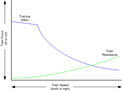
The first force is the tractive effort produced by the locomotive, whilst the second force is the resistance presented by the train. Whenever the tractive effort is greater than the train resistance the train will continue to move forward; once the resistance exceeds the tractive effort, then the train will start to slow down, and eventually will stop moving forward.

The sections below describe in more detail the forces of tractive effort and train resistance.

8.4.1.1.2. Train Resistance

The movement of the train is opposed by a number of different forces which are collectively grouped together to form the train resistance.

The main resistive forces are as follows (the first two values of resistance are modelled through the Davis formulas, and only apply on straight level track):

• Journal or Bearing resistance (or friction)
• Air resistance
• Gradient resistance – trains travelling up hills will experience greater resistive forces then those operating on level track.
• Curve resistance – applies when the train is traveling around a curve, and will be impacted by the curve radius, speed, and fixed wheel base of the rolling stock.
• Tunnel resistance – applies when a train is travelling through a tunnel.

8.4.1.1.3. Tractive Effort

Tractive Effort is created by the action of the steam against the pistons, which, through the media of rods, crossheads, etc., cause the wheels to revolve and the engine to advance.

Tractive Effort is a function of mean effective pressure of the steam cylinder and is expressed by following formula for a simple locomotive. Geared and compound locomotives will have slightly different formula:

TE = Cyl/2 x (M.E.P. x d2 x s) / D

Where:

• Cyl = number of cylinders
• TE = Tractive Effort (lbf)
• M.E.P. = mean effective pressure of cylinder (psi)
• D = diameter of cylinder (in)
• S = stroke of cylinder piston (in)
• D = diameter of drive wheels (in)

8.4.1.1.4. Theoretical Tractive Effort

To allow the comparison of different locomotives, as well as determining their relative pulling ability, a theoretical approximate value of tractive effort is calculated using the boiler gauge pressure and includes a factor to reduce the value of M.E.P.

Thus our formula from above becomes:

TE = Cyl/2 x (0.85 x BP x d2 x s) / D

Where:

• BP = Boiler Pressure (gauge pressure - psi)
• 0.85 – factor to account for losses in the engine, typically values between 0.7 and 0.85 were used by different manufacturers and railway companies.

8.4.1.1.5. Factor of Adhesion

The factor of adhesion describes the likelihood of the locomotive slipping when force is applied to the wheels and rails, and is the ratio of the starting Tractive Effort to the weight on the driving wheels of the locomotive:

FoA = Wd / TE

Where:

• FoA = Factor of Adhesion
• TE = Tractive Effort (lbs)
• Wd = Weight on Driving Wheels (lbs)

Typically the Factor of Adhesion should ideally be between 4.0 & 5.0 for steam locomotives. Values below this range will typically result in slippage on the rail.

8.4.1.1.6. Indicated HorsePower (IHP)

Indicated Horsepower is the theoretical power produced by a steam locomotive. The generally accepted formula for Indicated Horsepower is:

I.H.P. = Cyl/2 x (M.E.P. x L x A x N) / 33000

Where:

• IHP = Indicated Horsepower (hp)
• Cyl = number of cylinders
• M.E.P. = mean effective pressure of cylinder (psi)
• L = stroke of cylinder piston (ft)
• A = area of cylinder (sq in)
• N = number of cylinder piston strokes per min (NB: two piston strokes for every wheel revolution)

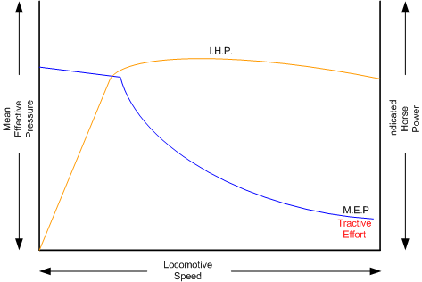
As shown in the diagram below, IHP increases with speed, until it reaches a maximum value. This value is determined by the cylinder’s ability to maintain an efficient throughput of steam, as well as for the boiler’s ability to maintain sufficient steam generation to match the steam usage by the cylinders.

8.4.1.1.7. Hauling Capacity of Locomotives

Thus it can be seen that the hauling capacity is determined by the summation of the tractive effort and the train resistance.

Different locomotives were designed to produce different values of tractive effort, and therefore the loads that they were able to haul would be determined by the track conditions, principally the ruling gradient for the section, and the load or train weight. Therefore most railway companies and locomotive manufacturers developed load tables for the different locomotives depending upon their theoretical tractive efforts.

The table below is a sample showing the hauling capacity of an American (4-4-0) locomotive from the Baldwin Locomotive Company catalogue, listing the relative loads on level track and other grades as the cylinder size, drive wheel diameter, and weight of the locomotive is varied.

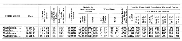
Typically the ruling gradient is defined as the maximum uphill grade facing a train in a particular section of the route, and this grade would typically determine the maximum permissible load that the train could haul in this section. The permissible load would vary depending upon the direction of travel of the train.

8.4.1.2. Elements of Steam Locomotive Operation

A steam locomotive is a very complex piece of machinery that has many component parts, each of which will influence the performance of the locomotive in different ways. Even at the peak of its development in the middle of the 20th century, the locomotive designer had at their disposal only a series of factors and simple formulae to describe its performance. Once designed and built, the performance of the locomotive was measured and adjusted by empirical means, i.e. by testing and experimentation on the locomotive. Even locomotives within the same class could exhibit differences in performance.

A simplified description of a steam locomotive is provided below to help understand some of the key basics of its operation.

As indicated above, the steam locomotive is a heat engine which converts fuel (coal, wood, oil, etc.) to heat; this is then used to do work by driving the pistons to turn the wheels. The operation of a steam locomotive can be thought of in terms of the following broadly defined components:

• Boiler and Fire (Heat conversion)
• Cylinder (Work done)

8.4.1.2.1. Boiler and Fire (Heat conversion)

The amount of work that a locomotive can do will be determined by the amount of steam that can be produced (evaporated) by the boiler.

Boiler steam production is typically dependent upon the Grate Area, and the Boiler Evaporation Area.

• Grate Area – the amount of heat energy released by the burning of the fuel is dependent upon the size of the grate area, draught of air flowing across the grate to support fuel combustion, fuel calorific value, and the amount of fuel that can be fed to the fire (a human fireman can only shovel so much coal in an hour). Some locomotives may have had good sized grate areas, but were ‘poor steamers’ because they had small draught capabilities.
• Boiler Evaporation Area – consisted of the part of the firebox in contact with the boiler and the heat tubes running through the boiler. This area determined the amount of heat that could be transferred to the water in the boiler. As a rule of thumb a boiler could produce approximately 12-15 lbs/h of steam per ft² of evaporation area.
• Boiler Superheater Area – Typically modern steam locomotives are superheated, whereas older locomotives used only saturated steam. Superheating is the process of putting more heat into the steam without changing the pressure. This provided more energy in the steam and allowed the locomotive to produce more work, but with a reduction in steam and fuel usage. In other words a superheated locomotive tended to be more efficient then a saturated locomotive.

8.4.1.2.2. Cylinder (Work done)

To drive the locomotive forward, steam was injected into the cylinder which pushed the piston backwards and forwards, and this in turn rotated the drive wheels of the locomotive. Typically the larger the drive wheels, the faster the locomotive was able to travel.

The faster the locomotive travelled the more steam that was needed to drive the cylinders. The steam able to be produced by the boiler was typically limited to a finite value depending upon the design of the boiler. In addition the ability to inject and exhaust steam from the cylinder also tended to reach finite limits as well. These factors typically combined to place limits on the power of a locomotive depending upon the design factors used.

8.4.1.3. Locomotive Types

During the course of their development, many different types of locomotives were developed, some of the more common categories are as follows:

• Simple – simple locomotives had only a single expansion cycle in the cylinder
• Compound – locomotives had multiple steam expansion cycles and typically had a high and low pressure cylinder.
• Saturated – steam was heated to only just above the boiling point of water.
• Superheated – steam was heated well above the boiling point of water, and therefore was able to generate more work in the locomotive.
• Geared – locomotives were geared to increase the tractive effort produced by the locomotive, this however reduced the speed of operation of the locomotive.

8.4.1.3.1. Superheated Locomotives

In the early 1900s, superheaters were fitted to some locomotives. As the name was implied a superheater was designed to raise the steam temperature well above the normal saturated steam temperature. This had a number of benefits for locomotive engineers in that it eliminated condensation of the steam in the cylinder, thus reducing the amount of steam required to produce the same amount of work in the cylinders. This resulted in reduced water and coal consumption in the locomotive, and generally improved the efficiency of the locomotive.

Superheating was achieved by installing a superheater element that effectively increased the heating area of the locomotive.

8.4.1.3.2. Geared Locomotives

In industrial type railways, such as those used in the logging industry, spurs to coal mines were often built to very cheap standards. As a consequence, depending upon the terrain, they were often laid with sharp curves and steep gradients compared to normal main line standards.

Typical main line rod type locomotives couldn’t be used on these lines due to their long fixed wheelbase (coupled wheels) and their relatively low tractive effort was no match for the steep gradients. Thus geared locomotives found their niche in railway practice.

Geared locomotives typically used bogie wheelsets, which allowed the rigid wheelbase to be reduced compared to that of rod type locomotives, thus allowing the negotiation of tight curves. In addition the gearing allowed an increase of their tractive effort to handle the steeper gradients compared to main line tracks.

Whilst the gearing allowed more tractive effort to be produced, it also meant that the maximum piston speed was reached at a lower track speed.

As suggested above, the maximum track speed would depend upon loads and track conditions. As these types of lines were lightly laid, excessive speeds could result in derailments, etc.

The three principal types of geared locomotives used were:

• Shay Locomotives
• Climax
• Heisler

8.4.2. Steam Locomotive Operation

To successfully drive a steam locomotive it is necessary to consider the performance of the following elements:

• Boiler and Fire (Heat conversion )
• Cylinder (Work done)

For more details on these elements, refer to the “Elements of Steam Locomotive Operation”

Summary of Driving Tips

• Wherever possible, when running normally, have the regulator at 100%, and use the reverser to adjust steam usage and speed.
• Avoid jerky movements when starting or running the locomotive, thus reducing the chances of breaking couplers.
• When starting always have the reverser fully wound up, and open the regulator slowly and smoothly, without slipping the wheels.

8.4.2.1. Open Rails Steam Functionality (Fireman)

The Open Rails Steam locomotive functionality provides two operational options:

• Automatic Fireman (Computer Controlled): In Automatic or Computer Controlled Fireman mode all locomotive firing and boiler management is done by Open Rails, leaving the player to concentrate on driving the locomotive. Only the basic controls such as the regulator and throttle are available to the player.
• Manual Fireman: In Manual Fireman mode all locomotive firing and boiler management must be done by the player. All of the boiler management and firing controls, such as blower, injector, fuel rate, are available to the player, and can be adjusted accordingly.

A full listing of the keyboard controls for use when in manual mode is provided on the Keyboard tab of the Open Rails Options panel.

Use the keys <Crtl+F> to switch between Manual and Automatic firing modes.

8.4.2.2. Hot or Cold Start

The locomotive can be started either in a hot or cold mode. Hot mode simulates a locomotive which has a full head of steam and is ready for duty.

Cold mode simulates a locomotive that has only just had the fire raised, and still needs to build up to full boiler pressure, before having full power available.

This function can be selected through the Open Rails options menu on the Simulation tab.

8.4.2.3. Main Steam Locomotive Controls

This section will describe the control and management of the steam locomotive based upon the assumption that the Automatic fireman is engaged. The following controls are those typically used by the driver in this mode of operation:

• Cylinder Cocks – allows water condensation to be exhausted from the cylinders. (Open Rails Keys: toggle <C>)
• Regulator – controls the pressure of the steam injected into the cylinders. (Open Rails Keys: <D> = increase, <A> = decrease)
• Reverser – controls the valve gear and when the steam is “cutoff”. Typically it is expressed as a fraction of the cylinder stroke. (Open Rails Keys: <W> = increase, <S> = decrease). Continued operation of the W or S key will eventually reverse the direction of travel for the locomotive.
• Brake – controls the operation of the brakes. (Open Rails Keys: <'> = increase, <;> = decrease)

8.4.2.3.1. Recommended Option Settings

For added realism of the performance of the steam locomotive, it is suggested that the following settings be considered for selection in the Open Rails options menu:

• Break couplers
• Curve speed dependent
• Curve resistance speed
• Hot start
• Tunnel resistance dependent

NB: Refer to the relevant sections of the manual for more detailed description of these functions.

8.4.2.3.2. Locomotive Starting

Open the cylinder cocks. They are to remain open until the engine has traversed a distance of about an average train length, consistent with safety.

The locomotive should always be started in full gear (reverser up as high as possible), according to the direction of travel, and kept there for the first few turns of the driving wheels, before adjusting the reverser.

After ensuring that all brakes are released, open the regulator sufficiently to move the train, care should be exercised to prevent slipping; do not open the regulator too much before the locomotive has gathered speed. Severe slipping causes excessive wear and tear on the locomotive, disturbance of the fire bed and blanketing of the spark arrestor. If slipping does occur, the regulator should be closed as appropriate, and if necessary sand applied.

Also, when starting, a slow even increase of power will allow the couplers all along the train to be gradually extended, and therefore reduce the risk of coupler breakages.

8.4.2.3.3. Locomotive Running

Theoretically, when running, the regulator should always be fully open and the speed of the locomotive controlled, as desired, by the reverser. For economical use of steam, it is also desirable to operate at the lowest cut-off values as possible, so the reverser should be operated at low values, especially running at high speeds.

When running a steam locomotive keep an eye on the following key parameters in the Heads up Display (HUD – <F5>) as they will give the driver an indication of the current status and performance of the locomotive with regard to the heat conversion (Boiler and Fire) and work done (Cylinder) processes. Also bear in mind the above driving tips.

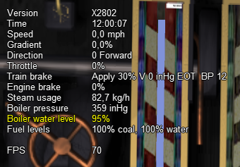
• Direction – indicates the setting on the reverser and the direction of travel. The value is in per cent, so for example a value of 50 indicates that the cylinder is cutting off at 0.5 of the stroke.
• Throttle – indicates the setting of the regulator in per cent.
• Steam usage – these values represent the current steam usage per hour.
• Boiler Pressure – this should be maintained close to the maximum working pressure of the locomotive.
• Boiler water level – indicates the level of water in the boiler. Under operation in Automatic Fireman mode, the fireman should manage this.
• Fuel levels – indicate the coal and water levels of the locomotive.

For information on the other parameters, such as the brakes, refer to the relevant sections in the manual.

For the driver of the locomotive the first two steam parameters are the key ones to focus on, as operating the locomotive for extended periods of time with steam usage in excess of the steam generation value will result in declining boiler pressure. If this is allowed to continue the locomotive will ultimately lose boiler pressure, and will no longer be able to continue to pull its load.

Steam usage will increase with the speed of the locomotive, so the driver will need to adjust the regulator, reverser, and speed of the locomotive to ensure that optimal steam pressure is maintained. However, a point will finally be reached where the locomotive cannot go any faster without the steam usage exceeding the steam generation. This point determines the maximum speed of the locomotive and will vary depending upon load and track conditions

The AI Fireman in Open Rails is not proactive, ie it cannot look ahead for gradients, etc, and therefore will only add fuel to the fire once the train is on the gradient. This reactive approach can result in a boiler pressure drop whilst the fire is building up. Similarly if the steam usage is dropped (due to a throttle decrease, such as approaching a station) then the fire takes time to reduce in heat, thus the boiler pressure can become excessive.

To give the player a little bit more control over this, and to facilitate the maintaining of the boiler pressure the following key controls have been added to the AI Fireman function:

AIFireOn - (<Alt+H>) - Forces the AI fireman to start building the fire up (increases boiler heat & pressure, etc) - typically used just before leaving a station to maintain pressure as steam consumption increases. This function will be turned off if AIFireOff, AIFireReset are triggered or if boiler pressure or BoilerHeat exceeds the boiler limit.

AIFireOff - (<Ctrl+H>) - Forces the AI fireman to stop adding to the fire (allows boiler heat to decrease as fire drops) - typically used approaching a station to allow the fire heat to decrease, and thus stopping boiler pressure from exceeding the maximum. This function will be turned off if AIFireOn, AIFireReset are triggered or if boiler pressure or BoilerHeat drops too low.

AIFireReset - (<Ctrl+Alt+H>) - turns off both of the above functions when desired.

If theses controls are not used, then the AI fireman operates in the same fashion as previously.

8.4.2.4. Steam Locomotive Carriage Steam Heat Modelling

8.4.2.4.1. Overview

In the early days of steam, passenger carriages were heated by fire burnt in stoves within the carriage, but this type of heating proved to be dangerous, as on a number of occasions the carriages actually caught fire and burnt.

A number of alternative heating systems were adopted as a safer replacement.

The Open Rails Model is based upon a direct steam model, ie one that has steam pipes installed in each carriage, and pumps steam into each car to raise the internal temperature in each car.

The heat model in each car is represented by Figure 1 below. The key parameters influencing the operation of the model are the values of tc, to, tp, which represent the temperature within the carriage, ambient temperature outside the carriage, and the temperature of the steam pipe due to steam passing through it.

As shown in the figure the heat model has a number of different elements as follows:

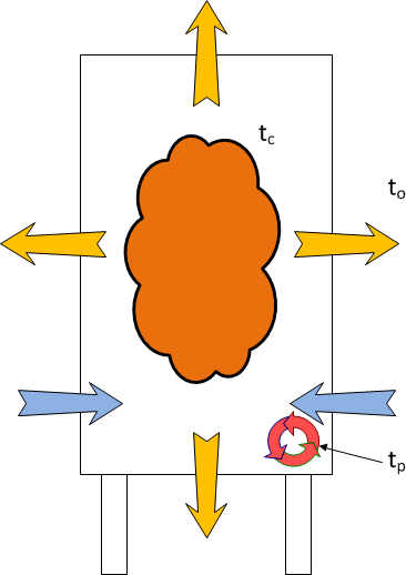
Heat Model for Passenger Car

1. Internal heat mass – the air mass in the carriage (represented by cloud) is heated to temperature that is comfortable to the passengers. The energy required to maintain the temperature will be determined the volume of the air in the carriage
2. Heat Loss – Transmission – over time heat will be lost through the walls, roof, and floors of the carriage (represented by outgoing orange arrows), this heat loss will reduce the temperature of the internal air mass.
3. Heat Loss – Infiltration – also over time as carriage doors are opened and closed at station stops, some cooler air will enter the carriage (represented by ingoing blue arrows), and reduce the temperature of the internal air mass.
4. Steam Heating – to offset the above heat losses, steam was piped through each of the carriages (represented by circular red arrows). Depending upon the heat input from the steam pipe, the temperature would be balanced by offsetting the steam heating against the heat losses.

8.4.2.4.2. Carriage Heating Implementation in Open Rails

Currently, carriage steam heating is only available on steam locomotives. To enable steam heating to work in Open Rails the following parameter must be included in the engine section of the steam locomotive ENG File:

MaxSteamHeatingPressure( x )

Where: x = maximum steam pressure in the heating pipe – should not exceed 100 psi

If the above parameter is added to the locomotive, then an extra line will appear in the extended HUD to show the temperature in the train, and the steam heating pipe pressure, etc.

Steam heating will only work if there are passenger cars attached to the locomotive.

Warning messages will be displayed if the temperature inside the carriage goes outside of the limits of 10–15.5°C.

The player can control the train temperature by using the following controls:

• <Alt+U> – increase steam pipe pressure (and hence train temperature)
• <Alt+D> – decrease steam pipe pressure (and hence train temperature)

The steam heating control valve can be configured by adding an enginecontroller called ORTSSTeamHeat ( w, x, y, z). It should be configured as a standard 4 value controller.

It should be noted that the impact of steam heating will vary depending upon the season, length of train, etc.

8.4.3. Steam Locomotives – Physics Parameters for Optimal Operation

8.4.3.1. Required Input ENG and WAG File Parameters

The OR Steam Locomotive Model (SLM) should work with default MSTS files; however optimal performance will only be achieved if the following settings are applied within the ENG file. The following list only describes the parameters associated with the SLM, other parameters such as brakes, lights, etc. still need to be included in the file. As always, make sure that you keep a backup of the original MSTS file.

Open Rails has been designed to do most of the calculations for the modeler, and typically only the key parameters are required to be included in the ENG or WAG file. The parameters shown in the Locomotive performance Adjustments section should be included only where a specific performance outcome is required, since default parameters should provide a satisfactory result.

When creating and adjusting ENG or WAG files, a series of tests should be undertaken to ensure that the performance matches the actual real-world locomotive as closely as possible. For further information on testing, as well as some suggested test tools, go to this site.

NB: These parameters are subject to change as Open Rails continues to develop.

Notes:

• New – parameter names starting with ORTS means added as part of OpenRails development
• Existing – parameter names not starting with ORTS are original in MSTS or added through MSTS BIN

Possible Locomotive Reference Info:

1. Steam Locomotive Data
2. Example Wiki Locomotive Data
3. Testing Resources for Open Rails Steam Locomotives

Parameter	Description	Recommended Units	Typical Examples
General Information (Engine section)
ORTS­Steam­Locomotive­Type ( x )	Describes the type of locomotive	Simple, Compound, Geared	(Simple) (Compound) (Geared)
Wheel­Radius ( x )	Radius of drive wheels	Distance	(0.648m) (36in)
Max­Steam­Heating­Pressure ( x )	Max pressure in steam heating system for passenger carriages	Pressure, NB: normally < 100 psi	(80psi)
Boiler Parameters (Engine section)
ORTS­Steam­Boiler­Type ( x )	Describes the type of boiler	Saturated, Superheated	(Saturated) (Superheated)
Boiler­Volume ( x )	Volume of boiler. This parameter is not overly critical.	Volume, where an act. value is n/a, use approx. EvapArea / 8.3	(“220*(ft^3)”) (“110*(m^3)”)
ORTS­Evaporation­Area ( x )	Boiler evaporation area	Area	(“2198*(ft^2)”) (“194*(m^2)”)
Max­Boiler­Pressure ( x )	Max boiler working pressure (gauge)	Pressure	(200psi) (200kPa)
ORTS­Superheat­Area ( x )	Superheating heating area	Area	(“2198*(ft^2)”) (“194*(m^2)” )
Locomotive Tender Info (Engine section)
Max­Tender­Water­Mass ( x )	Water in tender	Mass	(36500lb) (16000kg)
Max­Tender­Coal­Mass ( x )	Coal in tender	Mass	(13440lb) (6000kg)
Is­Tender­Required ( x )	Locomotive Requires a tender	0 = No, 1 = Yes	(0) (1)
Fire (Engine section)
ORTS­Grate­Area ( x )	Locomotive fire grate area	Area	(“2198*(ft^2)”) (“194*(m^2)”)
ORTS­Fuel­Calorific ( x )	Calorific value of fuel	For coal use 13700 btu/lb	(13700btu/lb) (33400kj/kg)
ORTS­Steam­Fireman­Max­Possible­Firing­Rate ( x )	Maximum fuel rate that fireman can shovel in an hour. (Mass Flow)	Use as def: UK:3000lb/h US:5000lb/h AU:4200lb/h	(4200lb/h) (2000kg/h)
Steam­Fireman­Is­Mechanical­Stoker ( x )	Mechanical stoker = large rate of coal feed	Boolean, 0=no-stoker 1=stoker	( 1 )
Steam Cylinder (Engine section)
Num­Cylinders ( x )	Number of steam cylinders	Boolean	( 2 )
Cylinder­Stroke ( x )	Length of cylinder stroke	Distance	(26in) (0.8m)
Cylinder­Diameter ( x )	Cylinder diameter	Distance	(21in) (0.6m)
LP­Num­Cylinders ( x )	Number of steam LP cylinders (compound locomotive only)	Boolean	( 2 )
LP­Cylinder­Stroke ( x )	LP cylinder stroke length (compound locomotive only)	Distance	(26in) (0.8m)
LP­Cylinder­Diameter ( x )	Diameter of LP cylinder (compound locomotive only)	Distance	(21in) (0.6m)
Friction (Wagon section)
ORTS­Davis_A ( x )	Journal or roller bearing + mechanical friction	N, lbf. Use FCalc to calculate	(502.8N) (502.8lb)
ORTS­Davis_B ( x )	Flange friction	Nm/s, lbf/mph. Use FCalc	(1.5465Nm/s) (1.5465lbf/mph)
ORTS­Davis_C ( x )	Air resistance friction	Nm/s^2, lbf/mph^2 Use FCalc	(1.43Nm/s^2) (1.43lbf/mph^2)
ORTS­Bearing­Type ( x )	Bearing type, defaults to Friction	Roller, Friction, Low	( Roller )
Friction (Engine section)
ORTS­Drive­Wheel­Weight ( x )	Total weight on the locomotive driving wheels	Mass, Leave out if unknown	(2.12t)
Curve Speed Limit (Wagon section)
ORTS­Unbalanced­Super­Elevation ( x )	Determines the amount of Cant Deficiency applied to carriage	Distance, Leave out if unknown	(3in) (0.075m)
ORTS­Track­Gauge( x )	Track gauge	Distance, Leave out if unknown	(4ft 8.5in) ( 1.435m ) ( 4.708ft)
Centre­Of­Gravity ( x, y, z )	Defines the centre of gravity of a locomotive or wagon	Distance, Leave out if unknown	(0m, 1.8m, 0m) (0ft, 5.0ft, 0ft)
Curve Friction (Wagon section)
ORTS­Rigid­Wheel­Base ( x )	Rigid wheel base of vehicle	Distance, Leave out if unknown	(5ft 6in) (3.37m)
Locomotive Gearing (Engine section – Only required if locomotive is geared)
ORTS­Steam­Gear­Ratio ( a, b )	Ratio of gears	Numeric	(2.55, 0.0)
ORTS­Steam­Max­Gear­Piston­Rate ( x )	Max speed of piston	ft/min	( 650 )
ORTS­Steam­Gear­Type ( x )	Fixed gearing or selectable gearing	Fixed, Select	(Fixed) (Select)
Locomotive Performance Adjustments (Engine section – Optional, for experienced modellers)
ORTS­Boiler­Evaporation­Rate ( x )	Multipl. factor for adjusting maximum boiler steam output	Be tween 10–15, Leave out if not used	(15.0)
ORTS­Burn­Rate ( x, y )	Tabular input: Coal combusted (y) to steam generated (x)	x – lbs, y – kg, series of x & y values. Leave out if unused
ORTS­Cylinder­Efficiency­Rate ( x )	Multipl. factor for steam cylinder (force) output	Un limited, Leave out if unused	(1.0)
ORTS­Boiler­Efficiency (x, y)	Tabular input: boiler efficiency (y) to coal combustion (x)	x – lbs/ft2/h, series of x & y values. Leave out if unused
ORTS­Cylinder­Exhaust­Open ( x )	Point at which the cylinder exhaust port opens	Between 0.1–0.95, Leave out if unused	(0.1)
ORTS­Cylinder­Port­Opening ( x )	Size of cylinder port opening	Between 0.05–0.12, Leave out if unused	(0.085)
ORTS­Cylinder­Initial­Pressure­Drop ( x, y )	Tabular input: wheel speed (x) to pressure drop factor (y)	x – rpm, series of x & y values. Leave out if unused
ORTS­Cylinder­Back­Pressure ( x, y )	Tabular input: Loco indicated power (x) to backpressure (y)	x – hp, y – psi(g), series of x & y values. Leave out if unused

8.4.4. Special Visual Effects for Locomotives or Wagons

Steam exhausts on a steam locomotive, and other special visual effects can be modelled in OR by defining appropriate visual effects in the SteamSpecialEffects section of the steam locomotive ENG file, the DieselSpecialEffects section of the diesel locomotive ENG file, or the SpecialEffects section of a relevant wagon (including diesel, steam or electric locomotives.

OR supports the following special visual effects in a steam locomotive:

• Steam cylinders (named CylindersFX and Cylinders2FX) – two effects are provided which will represent the steam exhausted when the steam cylinder cocks are opened. Two effects are provided to represent the steam exhausted at the front and rear of each piston stroke. These effects will appear whenever the cylinder cocks are opened, and there is sufficient steam pressure at the cylinder to cause the steam to exhaust, typically the regulator is open (> 0%).
• Stack (named StackFX) – represents the smoke stack emissions. This effect will appear all the time in different forms depending upon the firing and steaming conditions of the locomotive.
• Compressor (named CompressorFX) – represents a steam leak from the air compressor. Will only appear when the compressor is operating.
• Generator (named GeneratorFX) – represents the emission from the turbo-generator of the locomotive. This effect operates continually. If a turbo-generator is not fitted to the locomotive it is recommended that this effect is left out of the effects section which will ensure that it is not displayed in OR.
• Safety valves (named SafetyValvesFX) – represents the discharge of the steam valves if the maximum boiler pressure is exceeded. It will appear whenever the safety valve operates.
• Whistle (named WhistleFX) – represents the steam discharge from the whistle.
• Injectors (named Injectors1FX and Injectors2FX) – represents the steam discharge from the steam overflow pipe of the injectors. They will appear whenever the respective injectors operate.

OR supports the following special visual effects in a diesel locomotive:

• Exhaust (named Exhaustnumber) – is a diesel exhaust. Multiple exhausts can be defined, simply by adjusting the numerical value of the number after the key word exhaust.

OR supports the following special visual effects in a wagon (also the wagon section of an ENG file):

• Steam Heating Boiler (named HeatingSteamBoilerFX) – represents the exhaust for a steam heating boiler. Typically this will be set up on a diesel or electric train as steam heating was provided directly from a steam locomotive.
• Wagon Generator (named WagonGeneratorFX) – represents the exhaust for a generator. This generator was used to provide additional auxiliary power for the train, and could have been used for air conditioning, heating lighting, etc.
• Wagon Smoke (named WagonSmokeFX) – represents the smoke coming from say a wood fire. This might have been a heating unit located in the guards van of the train.
• Heating Hose (named HeatingHoseFX) – represents the steam escaping from a steam pipe connection between wagons.

NB: If a steam effect is not defined in the SteamSpecialEffects, DieselSpecialEffects, or the SpecialEffects section of an ENG/WAG file, then it will not be displayed in the simulation. Similarly if any of the co-ordinates are zero, then the effect will not be displayed.

Each effect is defined by inserting a code block into the ENG/WAG file similar to the one shown below:

CylindersFX (
    -1.0485 1.0 2.8
    -1  0  0
    0.1
)

The code block consists of the following elements:

• Effect name – as described above,
• Effect location on the locomotive (given as an x, y, z offset in metres from the origin of the wagon shape)
• Effect direction of emission (given as a normal x, y and z)
• Effect nozzle width (in metres)

8.4.5. Auxiliary Water Tenders

To increase the water carrying capacity of a steam locomotive, an auxiliary tender (or as known in Australia as a water gin) would sometimes be coupled to the locomotive. This auxiliary tender would provide additional water to the locomotive tender via connecting pipes.

Typically, if the connecting pipes were opened between the locomotive tender and the auxiliary tender, the water level in the two vehicles would equalise at the same height.

To implement this feature in Open Rails, a suitable water carrying vehicle needs to have the following parameter included in the WAG file.

ORTSAuxTenderWaterMass ( 70000lb ) The units of measure are in mass.

When the auxiliary tender is coupled to the locomotive the tender line in the LOCOMOTIVE INFORMATION HUD will show the two tenders and the water capacity of each. Water (C) is the combined water capacity of the two tenders, whilst Water (T) shows the water capacity of the locomotive tender, and Water (A) the capacity of the auxiliary tender (as shown below).

To allow the auxiliary tender to be filled at a water fuelling point, a water freight animation will be need to be added to the WAG file as well. (Refer to Freight Animations for more details).

8.5. Engines – Multiple Units in Same Consist or AI Engines

In an OR player train one locomotive is controlled by the player, while the other units are controlled by default by the train’s MU (multiple unit) signals for braking and throttle position, etc. The player-controlled locomotive generates the MU signals which are passed along to every unit in the train. For AI trains, the AI software directly generates the MU signals, i.e. there is no player-controlled locomotive. In this way, all engines use the same physics code for power and friction.

This software model will ensure that non-player controlled engines will behave exactly the same way as player controlled ones.

8.6. Open Rails Braking

Open Rails software has implemented its own braking physics in the current release. It is based on the Westinghouse 26C and 26F air brake and controller system. Open Rails braking will parse the type of braking from the .eng file to determine if the braking physics uses passenger or freight standards, self-lapping or not. This is controlled within the Options menu as shown in General Options above.

Selecting Graduated Release Air Brakes in Menu > Options allows partial release of the brakes. Some 26C brake valves have a cut-off valve that has three positions: passenger, freight and cut-out. Checked is equivalent to passenger standard and unchecked is equivalent to freight standard.

The Graduated Release Air Brakes option controls two different features. If the train brake controller has a self-lapping notch and the Graduated Release Air Brakes box is checked, then the amount of brake pressure can be adjusted up or down by changing the control in this notch. If the Graduated Release Air Brakes option is not checked, then the brakes can only be increased in this notch and one of the release positions is required to release the brakes.

Another capability controlled by the Graduated Release Air Brakes checkbox is the behavior of the brakes on each car in the train. If the Graduated Release Air Brakes box is checked, then the brake cylinder pressure is regulated to keep it proportional to the difference between the emergency reservoir pressure and the brake pipe pressure. If the Graduated Release Air Brakes box is not checked and the brake pipe pressure rises above the auxiliary reservoir pressure, then the brake cylinder pressure is released completely at a rate determined by the retainer setting.

The following brake types are implemented in OR:

• Vacuum single
• Air single-pipe
• Air twin-pipe
• EP (Electro-pneumatic)
• Single-transfer-pipe (air and vacuum)

The operation of air single-pipe brakes is described in general below.

The auxiliary reservoir needs to be charged by the brake pipe and, depending on the WAG file parameters setting, this can delay the brake release. When the Graduated Release Air Brakes box is not checked, the auxiliary reservoir is also charged by the emergency reservoir (until both are equal and then both are charged from the pipe). When the Graduated Release Air Brakes box is checked, the auxiliary reservoir is only charged from the brake pipe. The Open Rails software implements it this way because the emergency reservoir is used as the source of the reference pressure for regulating the brake cylinder pressure.

The end result is that you will get a slower release when the Graduated Release Air Brakes box is checked. This should not be an issue with two pipe air brake systems because the second pipe can be the source of air for charging the auxiliary reservoirs.

Open Rails software has modeled most of this graduated release car brake behavior based on the 26F control valve, but this valve is designed for use on locomotives. The valve uses a control reservoir to maintain the reference pressure and Open Rails software simply replaced the control reservoir with the emergency reservoir.

Increasing the Brake Pipe Charging Rate (psi/s) value controls the charging rate. Increasing the value will reduce the time required to recharge the train; while decreasing the value will slow the charging rate. However, this might be limited by the train brake controller parameter settings in the ENG file. The brake pipe pressure cannot go up faster than that of the equalization reservoir.

The default value, 21, should cause the recharge time from a full set to be about 1 minute for every 12 cars. If the Brake Pipe Charging Rate (psi/s) value is set to 1000, the pipe pressure gradient features will be disabled and will also disable some but not all of the other new brake features.

Brake system charging time depends on the train length as it should, but at the moment there is no modeling of main reservoirs and compressors.

8.6.1. Brake Shoe Adhesion

The braking of a train is impacted by the following two types of adhesion (friction coefficients):

• Brakeshoe – the coefficient of friction of the brakeshoe varies due to the type of brake shoe, and the speed of the wheel increases. Typically older cast iron brake shoes had lower friction coefficients then more modern composite brakeshoes.
• Wheel – the adhesion or friction coefficient between the wheel and the rail will also vary with different conditions, such as whether the track was dry or wet, and will also vary with the speed of rotation of the wheel.

Thus a train traveling at high speed will have lower brake shoe adhesion, which means that the train will take a longer time to stop (or alternatively more force needs to be applied to the brakeshoe to achieve the same slowing effect of the wheel, as at slower speeds). Traveling at high speeds may also result in insufficient force being available to stop the train, and therefore under some circumstances the train may become uncontrollable (unstoppable) or runaway on steep falling gradients.

Conversely if too much force is applied to the brakeshoe, then the wheel could lock up, and this could result in the wheel slipping along the rail once the adhesive force (wagon weight x coefficient of friction) of the wagon is exceeded by the braking force. In this instance the static friction between the wheel and the track will change to dynamic friction, which is significantly lower than the static friction, and thus the train will not be stopped in the desired time and distance.

When designing the braking forces railway engineers need to ensure that the maximum braking force applied to the wheels takes into account the above adhesion factors.

Implementation in Open Rails

Open Rails models the aspects described above, and operates within one of the following modes:

• Advanced Adhesion NOT selected - brake force operates as per previous OR functionality, i.e. - constant brake force regardless of speed.
• Advanced Adhesion SELECTED and legacy WAG files, or NO additional user friction data defined in WAG file - OR assumes the users assigned friction coefficient have been set at 20% friction coefficient for cast iron brakes, and reverse engineers the braking force, and then applies the default friction curve as the speed varies.
• Advanced Adhesion SELECTED and additional user friction data HAS been defined in WAG file - OR applies the user defined friction/speed curve.

It should be noted that the MaxBrakeForce parameter in the WAG file is the actual force applied to the wheel after reduction by the friction coefficient.

Option iii) above is the ideal recommended method of operating, and naturally will require include files, or variations to the WAG file.

To setup the WAG file, the following values need to be set:

• use the OR parameter ORTSBrakeShoeFriction ( x, y ) to define an appropriate friction/speed curve, where x = speed in kph, and y = brakeshoe friction. This parameter needs to be included in the WAG file near the section defining the brakes. This parameter allows the user to customise to any brake type.
• Define the MaxBrakeForce value with a friction value equal to the zero speed value of the above curve, i.e. in the case of the curve below this woyuld be 0.49.

For example, a sample curve definition for a COBRA (COmposition BRAkes) brakeshoe might be as follows:

ORTSBrakeShoeFriction ( 0.0 0.49 8.0 ................  80.5 0.298 88.5 0.295 96.6 0.289 104.6 0.288 )

The debug FORCES INFORMATION HUD has been modified by the addition of two extra columns:

• Brk. Frict. - Column shows the current friction value of the brakeshoe and will vary according to the speed. (Applies to modes ii) and iii) above). In mode i) it will show friction constant at 100%, which indicates that the MaxBrakeForce defined in the WAG file is being used without alteration, ie it is constant regardless of the speed.
• Brk. Slide - indicates that the vehicle wheels are sliding along the track under brake application. (Ref to Wheel Skidding due to Excessive Brake Force )

It should be noted that the Adhesion factor correction slider in the options menu will vary the brakeshoe coefficient above and below 100% (or unity). It is recommended that this is set @ the default value of 100%.

These changes introduce an extra challenge to train braking, but provide a more realistic train operation.

For example, in a lot of normal Westinghouse brake systems, a minimum pressure reduction was applied by moving the brake controller to the LAP position. Typically Westinghouse recommended values of between 7 and 10 psi.

8.6.2. Train Brake Pipe Losses

The train brake pipe on a train is subject to air losses through leakage at joints, etc. Typically when the brake controller is in the RUNNING position, air pressure is maintained in the pipe from the reservoir. However on some brake systems, especially older ones such as the A6-ET, when the brake controller is in the LAP position the train brkae pipe is isolated from the air reservoir, and hence over time the pipe will suffer pressure drops due to leakages. This will result in the brakes being gradually applied.

More modern brake systems have a self lapping feature which compensates for train brake pipe leakage regardless of the position that the brake controller is in.

Open Rails models this feature whenever the TrainPipeLeakRate parameter is defined in the engine section of the ENG file. Typically most railway companies accepted leakage rates of around 5 psi/min in the train brake pipe before some remedial action needed to be undertaken.

If this parameter is left out of the ENG file, then no leakage will occur.

8.6.3. Wheel Skidding due to Excessive Brake Force

The application of excessive braking force onto a wheel can cause it to lock up and then start to slip along the rails. This occurs where the wagon braking force exceeds the adhesive weight force of the wagon wheel, i.e. the wheel to rail friction is overcome, and the wheel no longer grips the rails.

Typically this happens with lightly loaded vehicles at lower speeds, and hence the need to ensure that braking forces are applied to design standards. Skidding will be more likely to occur when the adhesion between the wheel and track is low, so for example skidding is more likely in wet weather then dry weather. The value Wag Adhesion in the FORCES INFORMATION HUD indicates this adhesion value, and will vary with the relevant weather conditions.

When a vehicle experiences wheel skid, an indication is provided in the FORCES INFORMATION HUD. To correct the problem the brakes must be released, and then applied slowly to ensure that the wheels are not locked up. Wheel skid will only occur if ADVANCED adhesion is selected in the options menu.

(Ref to Wheel Skidding due to Excessive Brake Force for additional information)

8.6.4. Using the F5 HUD Expanded Braking Information

This helps users of Open Rails to understand the status of braking within the game and assists in realistically coupling and uncoupling cars. Open Rails braking physics is more realistic than MSTS, as it models the connection, charging and exhaust of brake lines.

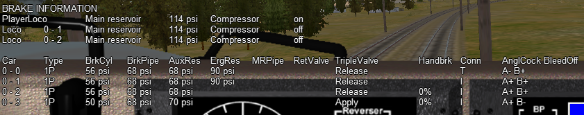
When coupling to a static consist, note that the brake line for the newly added cars normally does not have any pressure. This is because the train brake line/hose has not yet been connected. The last columns of each line shows the condition of the air brake hose connections of each unit in the consist.

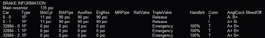
The columns under AnglCock describe the state of the Angle Cock, a manually operated valve in each of the brake hoses of a car: A is the cock at the front, B is the cock at the rear of the car. The symbol + indicates that the cock is open and the symbol - that it is closed. The column headed by T indicates if the hose on the locomotive or car is interconnected: T means that there is no connection, I means it is connected to the air pressure line. If the angle cocks of two consecutive cars are B+ and A+ respectively, they will pass the main air hose pressure between the two cars. In this example note that the locomotive air brake lines start with A- (closed) and end with B- (closed) before the air hoses are connected to the newly coupled cars. All of the newly coupled cars in this example have their angle cocks open, including those at the ends, so their brake pressures are zero. This will be reported as Emergency state.

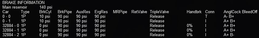
8.6.4.1. Coupling Cars

Also note that, immediately after coupling, you may also find that the handbrakes of the newly added cars have their handbrakes set to 100% (see column headed Handbrk). Pressing <Shift+;> (Shift plus semicolon in English keyboards) will release all the handbrakes on the consist as shown below. Pressing <Shift+'> (Shift plus apostrophe on English keyboards) will set all of the handbrakes. Cars without handbrakes will not have an entry in the handbrake column.

If the newly coupled cars are to be moved without using their air brakes and parked nearby, the brake pressure in their air hose may be left at zero: i.e. their hoses are not connected to the train’s air hose. Before the cars are uncoupled in their new location, their handbrakes should be set. The cars will continue to report State Emergency while coupled to the consist because their BC value is zero; they will not have any braking. The locomotive brakes must be used for braking. If the cars are uncoupled while in motion, they will continue coasting.

If the brakes of the newly connected cars are to be controlled by the train’s air pressure as part of the consist, their hoses must be joined together and to the train’s air hose and their angle cocks set correctly. Pressing the Backslash key <\>) (in English keyboards; please check the keyboard assignments for other keyboards) connects the brake hoses between all cars that have been coupled to the engine and sets the intermediate angle cocks to permit the air pressure to gradually approach the same pressure in the entire hose. This models the operations performed by the train crew. The HUD display changes to show the new condition of the brake hose connections and angle cocks:

All of the hoses are now connected; only the angle cocks on the lead locomotive and the last car are closed as indicated by the -. The rest of the cocks are open (+) and the air hoses are joined together (all I) to connect to the air supply on the lead locomotive.

Upon connection of the hoses of the new cars, recharging of the train brake line commences. Open Rails uses a default charging rate of about 1 minute per every 12 cars. The HUD display may report that the consist is in Emergency state; this is because the air pressure dropped when the empty car brake systems were connected. Ultimately the brake pressures reach their stable values:

If you don’t want to wait for the train brake line to charge, pressing <Shift+/> (in English keyboards) executes Brakes Initialize which will immediately fully charge the train brakes line to the final state. However, this action is not prototypical and also does not allow control of the brake retainers.

The state of the angle cocks, the hose connections and the air brake pressure of individual coupled cars can be manipulated by using the F9 Train Operations Monitor, described here. This will permit more realistic shunting of cars in freight yards.

8.6.4.2. Uncoupling Cars

When uncoupling cars from a consist, using the F5 HUD Expanded Brake Display in conjunction with the F9 Train Operations Monitor display allows the player to set the handbrakes on the cars to be uncoupled, and to uncouple them without losing the air pressure in the remaining cars. Before uncoupling, close the angle cock at the rear of the car ahead of the first car to be uncoupled so that the air pressure in the remaining consist is not lost when the air hoses to the uncoupled cars are disconnected. If this procedure is not followed, the train braking system will go into Emergency state and will require pressing the <\> (backslash) key to connect the air hoses correctly and then waiting for the brake pressure to stabilize again.

8.6.4.3. Setting Brake Retainers

If a long consist is to be taken down a long or steep grade the operator may choose to set the Brake Retainers on some or all of the cars to create a fixed braking force by those cars when the train brakes are released. (This requires that the retainer capability of the cars be enabled; either by the menu option Retainer valve on all cars, or by the inclusion of an appropriate keyword in the car’s .wag file.) The train must be fully stopped and the main brakes must be applied so that there is adequate pressure in the brake cylinders. Pressing <Shift+]> controls how many cars in the consist have their retainers set, and the pressure value that is retained when the train brakes are released. The settings are described in Brake Retainers below. Pressing <Shift+[> cancels the settings and exhausts all of the air from the brake cylinders when the brakes are released. The F5 display shows the symbol RV ZZ for the state of the retainer valve in all cars, where ZZ is: EX for Exhaust or LP or HP. When the system brakes are released and there are no retainers set, the air in the brake cylinders in the cars is normally released to the air. The BC pressure for the cars with retainers set will not fall below the specified value. In order to change the retainer settings, the train must be fully stopped. A sample F5 view with 50% LP is shown below:

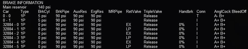
8.6.5. Dynamic Brakes

Open Rails software supports dynamic braking for engines. To increase the Dynamic brakes press Period (.) and Comma (,) to decrease them. Dynamic brakes are usually off at train startup (this can be overridden by the related MSTS setting in the .eng file), the throttle works and there is no value shown in the dynamic brake line in the HUD. To turn on dynamic brakes set the throttle to zero and then press Period. Pressing Period successively increases the Dynamic braking forces. If the value n in the MSTS parameter DynamicBrakesDelayTimeBeforeEngaging ( n ) is greater than zero, the dynamic brake will engage only after n seconds. The throttle will not work when the Dynamic brakes are on.

The Dynamic brake force as a function of control setting and speed can be defined in a DynamicBrakeForceCurves table that works like the MaxTractiveForceCurves table. If there is no DynamicBrakeForceCurves defined in the ENG file, than one is created based on the MSTS parameter values.

8.6.6. Native Open Rails Braking Parameters

Open Rails has implemented additional specific braking parameters to deliver realism in braking performance in the simulation.

Following are a list of specific OR parameters and their default values. The default values are used in place of MSTS braking parameters; however, two MSTS parameters are used for the release state: MaxAuxilaryChargingRate and EmergencyResChargingRate.

• wagon(brakepipevolume – Volume of car’s brake pipe in cubic feet (default .5). This is dependent on the train length calculated from the ENG to the last car in the train. This aggregate factor is used to approximate the effects of train length on other factors. Strictly speaking this value should depend on the car length, but the Open Rails Development team doesn’t believe it is worth the extra complication or CPU time that would be needed to calculate it in real time. We will let the community customize this effect by adjusting the brake servicetimefactor instead, but the Open Rails Development team doesn’t believe this is worth the effort by the user for the added realism.
• engine(mainreschargingrate – Rate of main reservoir pressure change in psi per second when the compressor is on (default .4).
• engine(enginebrakereleaserate – Rate of engine brake pressure decrease in psi per second (default 12.5).
• engine(enginebrakeapplicationrate – Rate of engine brake pressure increase in psi per second (default 12.5).
• engine(brakepipechargingrate – Rate of lead engine brake pipe pressure increase in PSI per second (default 21).
• engine(brakeservicetimefactor – Time in seconds for lead engine brake pipe pressure to drop to about 1/3 for service application (default 1.009).
• engine(brakeemergencytimefactor – Time in seconds for lead engine brake pipe pressure to drop to about 1/3 in emergency (default .1).
• engine(brakepipetimefactor – Time in seconds for a difference in pipe pressure between adjacent cars to equalize to about 1/3 (default .003).

8.6.7. Brake Retainers

The retainers of a car will only be available if either the General Option Retainer valve on all cars is checked, or the car’s .wag file contains a retainer valve declaration. To declare a retainer the line BrakeEquipmentType (  ) in the .wag file must include either the item Retainer_4_Position or the item Retainer_3_Position. A 4 position retainer includes four states: exhaust, low pressure (10 psi), high pressure (20 psi), and slow direct (gradual drop to zero). A 3 position retainer does not include the low pressure position. The use and display of the retainers is described in Extended HUD for Brake Information.

The setting of the retained pressure and the number of retainers is controlled using the Ctrl+[ and Ctrl+] keys (Ctrl plus the left and right square bracket ([ and ]) keys on an English keyboard). The Ctrl+[ key will reset the retainer on all cars in the consist to exhaust (the default position). Each time the Ctrl+] key is pressed the retainer settings are changed in a defined sequence. First the fraction of the cars set at a low pressure is selected (25%, 50% and then 100% of the cars), then the fraction of the cars at a high pressure is selected instead, then the fraction at slow direct. For the 25% setting the retainer is set on every fourth car starting at the rear of the train, 50% sets every other car and 100% sets every car. These changes can only be made when the train is stopped. When the retainer is set to exhaust, the ENG file release rate value is used, otherwise the pressures and release rates are hard coded based on some AB brake documentation used by the Open Rails development team.

8.6.8. Emergency Brake Application Key

The Backspace key is used, as in MSTS, to apply the train brakes in an emergency situation without requiring operation of the train brake lever. However in OR moving the brake lever back to the Release position will only cause OR to report Apply Emergency Brake Push Button. The Backspace key must be pressed again to cancel the emergency application, then normal operation can be resumed. When the button is active, the F5 HUD will display Emergency Brake Push Button in the Train Brake line.

8.6.9. Vacuum Brakes

Vacuum braking has been implemented in Open Rails in one of the two following forms:

• Direct Vacuum - in this form, while ever the Brake Pipe (BP) is connected to the ejectors or vacuum pump, depending upon the operating capacity of the ejectors, a vacuum will be maintained or created. Typically this will be when the brake controller is in a Brake Off position.
• Equalising Reservoir (EQ) - in this form a main vacuum reservoir is fitted to the locomotive, along with the equalising reservoir. Typically the main reservoir is maintained at a sufficiently high enough vacuum to create the vacuum in the BP to release the brakes. The BP vacuum will equalise at the vacuum set by the driver on the equalising reservoir.

In general, brakes (in particular a system with an equalising reservoir) will have three potential timings that impact the application or the releasing of the brakes.

1. In the equalising reservoir as the brake controller is varied
2. In the train brake pipe as the vacuum is increased or decreased
3. In the brake cylinder as it is applied or released.

In the case of brakes without an equalising reservoir only items ii) and iii) are valid in the above list.

The OR code attempts to model the above three items, however some compromises may need to be made, and it is suggested that the best outcome will be achieved when an overall timing approach is considered, rather than considering each of the individual components in isolation.

To enable the Equalising Reservoir option above BrakesTrainBrakeType must be set to vacuum_single_pipe_eq in the engine section of the ENG file.

Following is a list of specific OR parameters and their default values. The default values can be overwritten by including the following parameters into the relevant wagon section of the WAG or ENG file.

• wagon(BrakePipeVolume – Volume of brake pipe fitted to car in cubic feet (default calculated from car length, and assumption of 2in BP).
• wagon(ORTSAuxilaryResCapacity – Volume of auxiliary vacuum reservoir (coupled to brake cylinder) in cubic feet (default calculated on basis of 24in reservoir).
• wagon(ORTSBrakeCylinderSize – Size of brake cylinders fitted to wagon in inches (default assumes a 18in brake cylinder).
• wagon(ORTSNumberBrakeCylinders – Number of brake cylinders fitted to wagon, as an integer number (default 2).
• wagon(ORTSDirectAdmissionValve – Car has direct admission valves fitted, 0 = No, 1 = Yes (default No).
• wagon(ORTSBrakeShoeFriction – defines the friction curve for the brake shoe with speed (default curve for cast iron brake shoes included in OR).

Other standard brake parameters such as MaxBrakeForce, MaxReleaseRate , MaxApplicationRate, BrakeCylinderPressureForMaxBrakeBrakeForce can be used as well.

Additionaly the following are defined in the engine section of the ENG file:

• engine(ORTSBrakePipeChargingRate – sets the rate at which the brake pipe charges in InHg per second (default 0.32) This value should be calculated on the basis of feeding into a 200ft^3 brake system, as OR will adjust the value depending upon the connected volume of the brake cylinders and brake pipe.
• engine(ORTSBrakeServiceTimeFactor – Time for lead engine brake pipe pressure to drop in seconds (default 10.0)
• engine(ORTSBrakeEmergencyTimeFactor – Time for lead engine brake pipe pressure to drop under emergency conditions, in seconds (default 1.0)
• engine(ORTSBrakePipeTimeFactor – Controls propagation increase time along train pipe as vacuum increases, ie when brakes released, in seconds (default 0.02)
• engine(TrainPipeLeakRate – Rate at which the train brake pipe leaks at, in InHg per second (default no leakage)
• engine(ORTSVacuumBrakesMainResVolume – The volume of the main vacuum brake reservoir in cubic feet (default 110.0 , EQ operation only)
• engine(ORTSVacuumBrakesMainResMaxVacuum – The maximum vacuum in the main vacuum brake reservoir. When this pressure is reached the exhauster will automatically stop running, in InHg. (default 23 , EQ operation only)
• engine(ORTSVacuumBrakesExhausterRestartVacuum – pressure below which the exhauster will start to operate to recharge the main reservoir, in InHg (default 21 , EQ operation only)
• engine(ORTSVacuumBrakesMainResChargingRate – rate at which the main vacuum reservoir charges at, in InHg per second (default 0.2, EQ operation only)

Note: It is strongly recommended that UoM be used whenever units such as InHg, etc are specificed in the above parameters.

Other standard brake parameters such as VacuumBrakesHasVacuumPump, VacuumBrakesMinBoilerPressureMaxVacuum, VacuumBrakesSmallEjectorUsageRate, VacuumBrakesLargeEjectorUsageRate can be defined as well.

When defining the Brake Controllers for vacuum braked locomotives, only the following BrakesController tokens should be used - TrainBrakesControllerFullQuickReleaseStart, TrainBrakesControllerReleaseStart, TrainBrakesControllerRunningStart, TrainBrakesControllerApplyStart, TrainBrakesControllerHoldLappedStart, TrainBrakesControllerVacuumContinuousServiceStart, TrainBrakesControllerEmergencyStart, EngineBrakesControllerReleaseStart, EngineBrakesControllerRunningStart, EngineBrakesControllerApplyStart.

If TrainPipeLeakRate has been set in the ENG file, then the small ejector will be required to offset the leakage in the Brake Pipe. The J and Shft-J keys can be used to increase the level of operation of the small ejector.

An engine controller can be configured to customise the operation of the small ejector. This controller is called ORTSSmallEjector ( w, x, y, z ), and will be set up as a standard 4 value controller.

Engine brakes can also be configured for locomotives as required. They will work in a similar fashion to those fitted to air braked locomotives.

8.7. Dynamically Evolving Tractive Force

The Open Rails development team has been experimenting with max/continuous tractive force, where it can be dynamically altered during game play using the ORTSMaxTractiveForceCurves parameter as shown earlier. The parameters were based on the Handbook of Railway Vehicle Dynamics. This says the increased traction motor heat increase resistance which decreases current and tractive force. We used a moving average of the actual tractive force to approximate the heat in the motors. Tractive force is allowed to be at the maximum per the ENG file, if the average heat calculation is near zero. If the average is near the continuous rating than the tractive force is de-rated to the continuous rating. There is a parameter called ORTSContinuousForceTimeFactor that roughly controls the time over which the tractive force is averaged. The default is 1800 seconds.

8.8. Curve Resistance - Theory

8.8.1. Introduction

When a train travels around a curve, due to the track resisting the direction of travel (i.e. the train wants to continue in a straight line), it experiences increased resistance as it is pushed around the curve. Over the years there has been much discussion about how to accurately calculate curve friction. The calculation methodology presented (and used in OR) is meant to be representative of the impacts that curve friction will have on rolling stock performance.

8.8.2. Factors Impacting Curve Friction

A number of factors impact upon the value of resistance that the curve presents to the trains movement, as follows:

• Curve radius – the smaller the curve radius the higher the higher the resistance to the train
• Rolling Stock Rigid Wheelbase – the longer the rigid wheelbase of the vehicle, the higher the resistance to the train. Modern bogie stock tends to have shorter rigid wheelbase values and is not as bad as the older style 4 wheel wagons.
• Speed – the speed of the train around the curve will impact upon the value of resistance, typically above and below the equilibrium speed (i.e. when all the wheels of the rolling stock are perfectly aligned between the tracks). See the section below Impact of superelevation.

The impact of wind resistance on curve friction is calculated in the general calculations for Wind Resistance.

8.8.3. Impact of Rigid Wheelbase

The length of the rigid wheelbase of rolling stock will impact the value of curve resistance. Typically rolling stock with longer rigid wheelbases will experience a higher degree of rubbing or frictional resistance on tight curves, compared to stock with smaller wheelbases.

Steam locomotives usually created the biggest problem in regard to this as their drive wheels tended to be in a single rigid wheelbase as shown in figure. In some instances on routes with tighter curve the inside wheels of the locomotive were sometimes made flangeless to allow them to float across the track head. Articulated locomotives, such as Shays, tended to have their drive wheels grouped in bogies similar to diesel locomotives and hence were favoured for routes with tight curves.

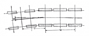
Diagram Source: The Baldwin Locomotive Works – Locomotive Data – 1944 Example of Rigid Wheelbase in steam locomotive

The value used for the rigid wheelbase is shown as W in figure

8.8.4. Impact of Super Elevation

On any curve whose outer rail is super-elevated there is, for any car, one speed of operation at which the car trucks have no more tendency to run toward either rail than they have on straight track, where both rail-heads are at the same level (known as the equilibrium speed). At lower speeds the trucks tend constantly to run down against the inside rail of the curve, and thereby increase the flange friction; whilst at higher speeds they run toward the outer rail, with the same effect. This may be made clearer by reference to figure below, which represents the forces which operate on a car at its centre of gravity.

With the car at rest on the curve there is a component of the weight W which tends to move the car down toward the inner rail. When the car moves along the track centrifugal force Fc comes into play and the car action is controlled by the force Fr which is the resultant of W and Fc. The force Fr likewise has a component which, still tends to move the car toward the inner rail. This tendency persists until, with increasing speed, the value of Fc becomes great enough to cause the line of operation of Fr to coincide with the centre line of the track perpendicular to the plane of the rails. At this equilibrium speed there is no longer any tendency of the trucks to run toward either rail. If the speed be still further increased, the component of Fr rises again, but now on the opposite side of the centre line of the track and is of opposite sense, causing the trucks to tend to move toward the outer instead of the inner rail, and thereby reviving the extra flange friction. It should be emphasized that the flange friction arising from the play of the forces here under discussion is distinct from and in excess of the flange friction which arises from the action of the flanges in forcing the truck to follow the track curvature. This excess being a variable element of curve resistance, we may expect to find that curve resistance reaches a minimum value when this excess reduces to zero, that is, when the car speed reaches the critical value referred to. This critical speed depends only on the super-elevation, the track gauge, and the radius of the track curvature. The resulting variation of curve resistance with speed is indicated in diagram below.

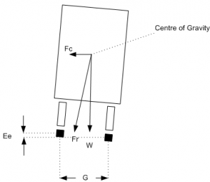
Forces on rolling stock transitioning a curve

8.8.5. Calculation of Curve Resistance

R = W F (D + L) 2 r

Where:

• R = Curve resistance,
• W = vehicle weight,
• F = Coefficient of Friction,
• μ = 0.5 for dry, smooth steel-to-steel; wet rail 0.1 – 0.3,
• D = track gauge,
• L = Rigid wheelbase,
• r = curve radius.

(Source: The Modern locomotive by C. Edgar Allen - 1912)

8.8.6. Calculation of Curve Speed Impact

The above value represents the least value amount of resistance, which occurs at the equilibrium speed, and as described above will increase as the train speed increases and decreases from the equilibrium speed. This concept is shown pictorially in the following graph. Open Rails uses the following formula to model the speed impact on curve resistance:

\[SpeedFactor = abs\left(\left(v_{equilibrium} - v_{train}\right) \cdot v_{equilibrium}\right)\cdot ResistanceFactor_{start}\]

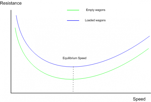
Generalisation of Variation of Curve Resistance With Speed

8.8.7. Further background reading

http://en.wikipedia.org/wiki/Curve_resistance_(railroad)

8.9. Curve Resistance - Application in OR

Open Rails models this function, and the user may elect to specify the known wheelbase parameters, or the above standard default values will be used. OR calculates the equilibrium speed in the speed curve module, however it is not necessary to select both of these functions in the simulator options TAB. Only select the function desired. By studying the Forces Information table in the HUD, you will be able to observe the change in curve resistance as the speed, curve radius, etc. vary.

8.9.1. OR Parameter Values

Typical OR parameter values may be entered in the Wagon section of the .wag or .eng file, and are formatted as below.:

ORTSRigidWheelBase ( 3in )
ORTSTrackGauge ( 4ft 8.5in) // (also used in curve speed module)

8.9.2. OR Default Values

The above values can be entered into the relevant files, or alternatively if they are not present, then OR will use the default values described below.

Rigid Wheelbase – as a default OR uses the figures shown above in the Typical Rigid Wheelbase Values section. The starting curve resistance value has been assumed to be 200%, and has been built into the speed impact curves. OR calculates the curve resistance based upon the actual wheelbases provided by the player or the appropriate defaults. It will use this as the value at Equilibrium Speed, and then depending upon the actual calculated equilibrium speed (from the speed limit module) it will factor the resistance up as appropriate to the current train speed.

Steam locomotive wheelbase approximation – the following approximation is used to determine the default value for the fixed wheelbase of a steam locomotive.

\[WheelBase = 1.25\cdot(axles - 1)\cdot DrvWheelDiameter\]

8.9.3. Typical Rigid Wheelbase Values

The following values are used as defaults where actual values are not provided by the player.

Rolling Stock Type	Typical value
Freight Bogie type stock (2 wheel bogie)	5’ 6” (1.6764m)
Passenger Bogie type stock (2 wheel bogie)	8’ (2.4384m)
Passenger Bogie type stock (3 wheel bogie)	12’ (3.6576m)
Typical 4 wheel rigid wagon	11’ 6” (3.5052m)
Typical 6 wheel rigid wagon	12’ (3.6576m)
Tender (6 wheel)	14’ 3” (4.3434m)
Diesel, Electric Locomotives	Similar to passenger stock
Steam locomotives	Dependent on drive wheels #. Can be up to 20’+, e.g. large 2–10–0 locomotives

Modern publications suggest an allowance of approximately 0.8 lb per ton (US) per degree of curvature for standard gauge tracks. At very slow speeds, say 1 or 2 mph, the curve resistance is closer to 1.0 lb (or 0.05% up grade) per ton per degree of curve.

8.10. Super Elevation (Curve Speed Limit) – Theory

8.10.1. Introduction

When a train rounds a curve, it tends to travel in a straight direction and the track must resist this movement, and force the train to move around the curve. The opposing movement of the train and the track result in a number of different forces being in play.

8.10.2. 19th & 20th Century vs Modern Day Railway Design

In the early days of railway construction financial considerations were a big factor in route design and selection. Given that the speed of competing transport, such as horses and water transport was not very great, speed was not seen as a major factor in the design process. However as railway transportation became a more vital need for society, the need to increase the speed of trains became more and more important. This led to many improvements in railway practices and engineering. A number of factors, such as the design of the rolling stock, as well as the track design, ultimately influence the maximum speed of a train. Today’s high speed railway routes are specifically designed for the speeds expected of the rolling stock.

8.10.3. Centrifugal Force

Railway locomotives, wagons and carriages, hereafter referred to as rolling stock, when rounding a curve come under the influence of centrifugal force. Centrifugal force is commonly defined as:

• The apparent force that is felt by an object moving in a curved path that acts outwardly away from the centre of rotation.
• An outward force on a body rotating about an axis, assumed equal and opposite to the centripetal force and postulated to account for the phenomena seen by an observer in the rotating body.

For this article the use of the phrase centrifugal force shall be understood to be an apparent force as defined above.

8.10.4. Effect of Centrifugal Force

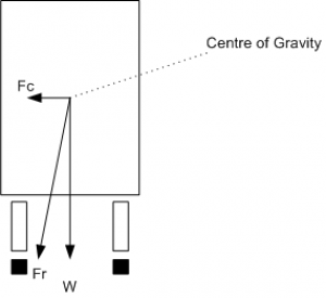
Forces at work when a train rounds a curve

When rolling stock rounds a curve, if the rails of the track are at the same elevation (i.e. the two tracks are at the same level) the combination of centrifugal force Fc and the weight of the rolling stock W will produce a resulting force Fr that does not coincide with the centre line of track, thus producing a downward force on the outside rail of the curve that is greater than the downward force on the inside rail (Refer to Figure 1). The greater the velocity and the smaller the radius of the curve (some railways have curve radius as low as 100m), the farther the resulting force Fr will move away from the centre line of track. Equilibrium velocity was the velocity at which a train could negotiate a curve with the rolling stock weight equally distributed across all the wheels.

If the position of the resulting force Fr approaches the outside rail, then the rolling stock is at risk of falling off the track or overturning. The following drawing, illustrates the basic concept described. Lateral displacement of the centre of gravity permitted by the suspension system of the rolling stock is not illustrated.

8.10.5. Use of Super Elevation

This illustrates the concept.

In order to counteract the effect of centrifugal force Fc the outside rail of the curve may be elevated above the inside rail, effectively moving the centre of gravity of the rolling stock laterally toward the inside rail.

This procedure is generally referred to as super elevation. If the combination of lateral displacement of the centre of gravity provided by the super elevation, velocity of the rolling stock and radius of curve is such that resulting force Fr becomes centred between and perpendicular to a line across the running rails the downward pressure on the outside and inside rails of the curve will be the same. The super elevation that produces this condition for a given velocity and radius of curve is known as the balanced or equilibrium elevation.

8.10.6. Limitation of Super Elevation in Mixed Passenger & Freight Routes

Typical early railway operation resulted in rolling stock being operated at less than equilibrium velocity (all wheels equally sharing the rolling stock weight ), or coming to a complete stop on curves. Under such circumstances excess super elevation may lead to a downward force sufficient to damage the inside rail of the curve, or cause derailment of rolling stock toward the centre of the curve when draft force is applied to a train. Routine operation of loaded freight trains at low velocity on a curve superelevated to permit operation of higher velocity passenger trains will result in excess wear of the inside rail of the curve by the freight trains.

Thus on these types of routes, super elevation is generally limited to no more than 6 inches.

8.10.7. Limitation of Super Elevation in High Speed Passenger Routes

Modern high speed passenger routes do not carry slower speed trains, nor expect trains to stop on curves, so it is possible to operate these routes with higher track super elevation values. Curves on these types of route are also designed with a relatively gentle radius, and are typically in excess of 2000m (2km) or 7000m (7km) depending on the speed limit of the route.

Parameters	France	Germany	Spain	Korea	Japan
Speed (km/h)	300/350	300	350	300/350	350
Horizontal curve radius (m)	10000 (10km)	7000 (7km)	7000 (7km)	7000 (7km)	4000 (4km)
Super elevation (mm)	180	170	150	130	180
Max Grade (mm/m)	35	40	12.5	25	15
Cant Gradient (mm/s)	50	34.7	32	N/A	N/A
Min Vertical radius (m)	16000 (16km)	14000 (14km)	24000 (24km)	N/A	10000 (10km)

Table: Curve Parameters for High Speed Operations (Railway Track Engineering by J. S. Mundrey)

8.10.8. Maximum Curve Velocity

The maximum velocity on a curve may exceed the equilibrium velocity, but must be limited to provide a margin of safety before overturning velocity is reached or a downward force sufficient to damage the outside rail of the curve is developed. This velocity is generally referred to as maximum safe velocity or safe speed. Although operation at maximum safe velocity will avoid overturning of rolling stock or rail damage, a passenger riding in a conventional passenger car will experience centrifugal force perceived as a tendency to slide laterally on their seat, creating an uncomfortable sensation of instability. To avoid passenger discomfort, the maximum velocity on a curve is therefore limited to what is generally referred to as maximum comfortable velocity or comfortable speed. Operating experience with conventional passenger cars has led to the generally accepted practice, circa 1980, of designating the maximum velocity for a given curve to be equal to the result for the calculation of equilibrium velocity with an extra amount added to the actual super elevation that will be applied to the curve. This is often referred to as unbalanced super elevation or cant deficiency. Tilt trains have been introduced to allow faster train operation on tracks not originally designed for high speed operation, as well as high speed railway operation. The tilting of the passenger cab allows greater values of unbalanced super elevation to be used.

8.10.9. Limitation of Velocity on Curved Track at Zero Cross Level

The concept of maximum comfortable velocity may also be used to determine the maximum velocity at which rolling stock is permitted to round curved track without super elevation and maintained at zero cross level. The lead curve of a turnout located between the heel of the switch and the toe of the frog is an example of curved track that is generally not super elevated. Other similar locations would include yard tracks and industrial tracks where the increased velocity capability made possible by super elevation is not required. In such circumstances the maximum comfortable velocity for a given curve may also be the maximum velocity permitted on tangent track adjoining the curve.

8.10.10. Height of Centre of Gravity

Operation on a curve at equilibrium velocity results in the centre of gravity of the rolling stock coinciding with a point on a line that is perpendicular to a line across the running rails and the origin of which is midway between the rails. Under this condition the height of the centre of gravity is of no consequence as the resulting force Fr coincides with the perpendicular line described above. When rolling stock stops on a super elevated curve or rounds a curve under any condition of non-equilibrium the resulting force Fr will not coincide with the perpendicular line previously described and the height of the centre of gravity then becomes significant in determining the location of the resulting force Fr relative to the centre line of the track. The elasticity of the suspension system of rolling stock under conditions of non-equilibrium will introduce a roll element that affects the horizontal displacement of the centre of gravity and that must also be considered when determining the location of the resulting force Fr.

8.10.11. Calculation of Curve Velocity

The generic formula for calculating the various curve velocities is as follows:

\[v = \sqrt{E\cdot g\cdot r\cdot G}\]

Where:

• E = Ea (track super elevation) + Ec (unbalanced super elevation)
• g = acceleration due to gravity
• r = radius of curve
• G = track gauge

8.10.12. Typical Super Elevation Values & Speed Impact – Mixed Passenger & Freight Routes

The values quoted below are “typical” but may vary from country to country.

Track super elevation typically will not be more than 6 inches (150mm). Naturally, depending upon the radius of the curve, speed restrictions may apply.

Normally unbalanced super elevation is typically restricted to 3 inches (75mm), and is usually only allowed for passenger stock.

Tilt trains may have values of up to 12 inches (305mm).

8.10.13. Typical Super Elevation Values & Speed Impact – High Speed Passenger Routes

	Cant D (SuperElevation) (mm)	Cant deficiency (Unbalanced SuperElevation) I (mm)
CEN (draft) – Tilting trains	180–200	300
Czech Rep. – Tilting trains	150	270
France – Tilting trains	180	260
Germany – Tilting trains	180	300
Italy – Tilting trains	160	275
Norway – Tilting trains	150	280
Spain – Tilting trains (equivalent for standard gauge)	160 (139)	210 (182)
Sweden – Tilting trains	150	245
UK – Tilting trains	180	300

Table: Super Elevation limits (source - Tracks for tilting trains - A study within the Fast And Comfortable Trains (FACT) project by B. Kufver, R. Persson)

8.11. Super Elevation (Curve Speed Limit) Application in OR

Open Rails implements this function, and has standard default values applied. The user may elect to specify some of the standard parameters used in the above formula.

8.11.1. OR Super Elevation Parameters

Typical OR parameters can be entered in the Wagon section of the .wag or .eng file, and are formatted as below.

ORTSUnbalancedSuperElevation ( 3in )
ORTSTrackGauge( 4ft 8.5in)

8.11.2. OR Super Elevation Default Values

The above values can be entered into the relevant files, or alternatively OR will default to the following functionality.

OR will initially use the speed limit value from the route’s .trk file to determine whether the route is a conventional mixed freight and passenger route or a high speed route.

• Speed limit < 200km/h (125mph) – Mixed Freight and Pass route
• Speed limit > 200km/h (125mph) – High speed passenger route

Default values of tracksuperelevation will be applied based upon the above classifications.

Track gauge will default to the standard value of 4’ 8.5” (1435mm).

Unbalancedsuperelevation (Cant Deficiency) will be determined from the value entered by the user, or will default to the following values:

• Conventional Freight – 0” (0mm)
• Conventional Passenger – 3” (75mm)
• Engines & tenders – 6” (150mm)

Tilting trains require the addition of the relevant unbalancedsuperelevation information to the relevant rolling stock files.

8.12. Tunnel Friction – Theory

8.12.1. Introduction

When a train travels through a tunnel it experiences increased resistance to the forward movement.

Over the years there has been much discussion about how to accurately calculate tunnel resistance. The calculation methodology presented (and used in OR) is meant to provide an indicative representation of the impacts that tunnel resistance will have on rolling stock performance.

8.12.2. Factors Impacting Tunnel Friction

In general, the train aerodynamics are related to aerodynamic drag, pressure variations inside the train, train-induced flows, cross-wind effects, ground effects, pressure waves inside the tunnel, impulse waves at the exit of tunnel, noise and vibration, etc. The aerodynamic drag is dependent on the cross-sectional area of the train body, train length, the shape of train fore- and after-bodies, the surface roughness of train body, and geographical conditions around the traveling train. The train-induced flows can influence passengers on a subway platform and is also associated with the cross-sectional area of the train body, the train length, the shape of train fore- and after-bodies, surface roughness of train body, etc.

A high speed train entering a tunnel generates a compression wave at the entry portal that moves at the speed of sound in front of the train. The friction of the displaced air with the tunnel wall produces a pressure gradient and, as a consequence, a rise in pressure in front of the train. On reaching the exit portal of the tunnel, the compression wave is reflected back as an expansion wave but part of it exits the tunnel and radiates outside as a micro-pressure wave. This wave could cause a sonic boom that may lead to structural vibration and noise pollution in the surrounding environment. The entry of the tail of the train into the tunnel produces an expansion wave that moves through the annulus between the train and the tunnel. When the expansion pressure wave reaches the entry portal, it is reflected towards the interior of the tunnel as a compression wave. These compression and expansion waves propagate backwards and forwards along the tunnel and experience further reflections when meeting with the nose and tail of the train or reaching the entry and exit portals of the tunnel until they eventually dissipate completely.

The presence of this system of pressure waves in a tunnel affects the design and operation of trains, and they are a source of energy losses, noise, vibrations and aural discomfort for passengers.

These problems are even worse when two or more trains are in a tunnel at the same time. Aural comfort is one of the major factors determining the area of new tunnels or the maximum train speed in existing tunnels.

8.12.3. Importance of Tunnel Profile

As described above, a train travelling through a tunnel will create a bow wave of air movement in front of it, which is similar to a piston effect. The magnitude and impact of this effect will principally be determined by the tunnel profile, train profile and speed.

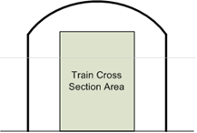
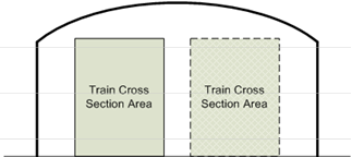
Typical tunnel profiles are shown in the diagrams.

As can be seen from these diagrams, the smaller the tunnel cross sectional area compared to the train cross sectional area, the less air that can escape around the train, and hence the greater the resistance experienced by the train. Thus it can be understood that a single train in a double track tunnel will experience less resistance then a single train in a single track tunnel.

8.12.4. Calculation of Tunnel Resistance

\[W_t = \frac{AL_{tr}}{(P + G)}v^2 \left(1 - \frac{1}{1+\sqrt{\frac{B+C(L_t - L_{tr})}{L_{tr}}}}\right)^2\]

where

\[ \begin{align}\begin{aligned}A=\frac{0.00003318\cdot\rho\cdot F_t}{(1-F_{tr}/F_t)^2},\\B=174.419(1-F_{tr}/F_t)^2,\\C=2.907\frac{(1-F_{tr}/F_t)^2}{4F_t/R_t}.\end{aligned}\end{align} \]

Ft – tunnel cross-sectional area (m2)	Ftr – train cross-sectional area (m2)
ρ – density of air ( = 1.2 kg/m3)	Rt – tunnel perimeter (m)
Ltr – length of train (m)	Lt – length of tunnel (m)
v – train velocity (m/s)	P – locomotive mass (t)
Wt – additional aerodynamic drag in tunnel (N/kN)	G – train mass (t)

Source: Reasonable compensation coefficient of maximum gradient in long railway tunnels by Sirong YI*, Liangtao NIE, Yanheng CHEN, Fangfang QIN

8.13. Tunnel Friction – Application in OR

To enable this calculation capability it is necessary to select the Tunnel dependent resistance option on the Open Rails Menu. The implication of tunnel resistance is designed to model the relative impact, and does not take into account multiple trains in the tunnel at the same time.

Tunnel resistance values can be seen in the Train Forces HUD.

The default tunnel profile is determined by the route speed recorded in the TRK file.

8.13.1. OR Parameters

The following parameters maybe included in the TRK file to overwrite standard default values used by Open Rails:

• ORTSSingleTunnelArea ( x ) – Cross section area of single track tunnel – units area
• ORTSSingleTunnelPerimeter ( x ) – Perimeter of single track tunnel – units distance
• ORTSDoubleTunnelArea ( x ) – Cross section area of double track tunnel – units area
• ORTSDoubleTunnelPerimeter ( x ) – Perimeter of double track tunnel – units distance

To insert these values in the .trk file, it is suggested that you add them just prior to the last parenthesis. You may also use an Include file method, described here.

8.13.2. OR Defaults

Open Rails uses the following standard defaults, unless overridden by values included in the TRK file.

Speed	1 track	2 tracks
Tunnel Perimeter
< 160 km/h	21.3 m	31.0 m
160 < 200 km/h	25.0 m	34.5 m
200 < 250 km/h	28.0 m	35.0 m
250 < 350 km/h	32.0 m	37.5 m
Tunnel Cross Sectional Area
< 120 km/h	27.0 m2	45.0 m2
< 160 km/h	42.0 m2	76.0 m2
200 km/h	50.0 m2	80.0 m2
250 km/h	58.0 m2	90.0 m2
350 km/h	70.0 m2	100.0 m2

8.14. Wind Resistance

The default Davis resistance formula is only valid for train operation in STILL air. At high train speeds, and especially for Very Fast trains the impact of wind can be quite significant, and special consideration is required when designing rolling stock, etc. If wind is present, then the impact of drag forces on the train will vary, and be in addition to the values calculated in the default (or still air) conditions.

The wind resistance in OR is modeled by the following two components:

Wind Drag Resistance - If a train is heading into a headwind then the train will experience greater resistance to movement, similarly if the train has a tailwind, then the trains resistance will decrease as the wind provides a “helping hand”. As the wind swings from the head of the train to the rear resistance will decrease. When the wind is perpendicular to the train, drag impact due to the wind will be zero.

Wind Lateral Force Resistance - When the wind blows from the side of the train, the train will be pushed against the outside track rail, thus increasing the amount of resistance experienced by the train.

To activate calculation of wind resistance, select the tickbox for “Wind dependent resistance” in the Simulation TAB of the options menu. As wind only becomes significant at higher train speeds, the wind resistance calculation only commences once the train speed exceeds 5 mph.

The amount of wind resistance that the train is experiencing is shown in the FORCES INFORMATION HUD. (see attached screenshot) The current wind conditions are also shown in the HUD, and include the Wind speed and direction, train direction, and the resulting vectors for the combined train and wind speed. The value in the Friction column is the default still air conditions as calculated by the Davis formula. It should be noted that OR calculates the Wind Drag resistance as a difference compared to the still air Davis C value, and hence it is possible for values in the Wind column to go negative on occasions. This is most likely when the wind is blowing from the rear of the train, ie the ResWind direction is greater then 90°C degrees, and hence the wind is actually aiding the train movement, and in effect reducing the amount of still air resistance.

The wind model has been adjusted in the following way:

• Wind Update speed - 1 sec
• Wind direction will always be within +/- 45°C degrees of the randomly selected default value selected at startup
• Wind speed is limited to approx 10mph.

The Wind Resistance model will use default information, such as the width and height of the stock from the Size statement, so by default it is not necessary to add any additional parameters for its operation. However for those who like to customise, the following parameters can be inputted via the WAG file or section.

ORTSWagonFrontalArea – The frontal cross sectional area of the wagon. The default units are in ft^2, so if entering metres, include the Units of Measure.

ORTSDavisDragConstant – OR by default uses the standard Davis Drag constants. If alternate drag constants are used in calculating the still air resistance, then it might be worthwhile inputting these values.

8.15. Trailing Locomotive Resistance

Typically only one set of resistance parameters is allowed for each WAG file. In the case of locomotives this can create issues as a leading locomotive will have a higher drag resistance then a trailing locomotive.

OR automatically adjusts the Drag resistance for trailing locomotives based upon the ratio of the original Davis formula.

However for those who like to customise, the following parameter can be inputted via the WAG file or section.

ORTSTrailLocomotiveResistanceFactor – The constant value by which the leading locomotive resistance needs to be decreased for trailing operation.

For steam locomotive tenders it may be necessary to enter this value depending upon the Drag constant used to calculate the tender resistance.

8.16. OR-Specific Include Files for Modifying MSTS File Parameters

8.16.1. Modifications to .eng and .wag Files

In the preceding paragraphs many references have been made to OR-specific parameters and tables to be included in .eng and .wag files. MSTS is in general quite tolerant if it finds unknown parameters and even blocks within .eng and .wag files, and continues running normally. However this way of operating is not encouraged by the OR team. Instead, a cleaner approach, as described here, has been implemented.

Within the trainset folder containing the .eng and .wag files to be upgraded, create a subfolder named OpenRails. Only OR will read files from this folder. Within this subfolder a text file named xxxx.eng or xxxx.wag, where xxxx.eng or xxxx.wag is the name of the original file, must be created.

This new file may contain either:

• all of the information included in the original file (using (modified parts where desired) plus the OR-specific parts if any, or:
• at its beginning only an include reference to the original file, followed by the modified parts and the OR-specific parts. This does not apply to the Name() statement and the Loco Description Information, where in any case the data in the base .eng file is retained.

An example of an OR-specific bc13ge70tonner.eng file to be placed into the OpenRails subfolder that uses the second possibility is as follows:

include ( ../bc13ge70tonner.eng )
Wagon (
  MaxReleaseRate ( 2.17 )
  MaxApplicationRate ( 3.37 )
  MaxAuxilaryChargingRate ( .4 )
  EmergencyResChargingRate ( .4 )
  BrakePipeVolume ( .4 )
  ORTSUnbalancedSuperElevation ( 3in )
Engine (
  AirBrakeMainresvolume ( 16 )
  MainResChargingRate ( .5 )
  BrakePipeChargingRate ( 21 )
  EngineBrakeReleaseRate ( 12.5 )
  EngineBrakeApplicationRate ( 12.5 )
  BrakePipeTimeFactor ( .00446 )
  BrakeServiceTimeFactor ( 1.46 )
  BrakeEmergencyTimeFactor ( .15 )
  ORTSMaxTractiveForceCurves (
    0 (
      0 0 50 0 )
    .125 (
      0 23125
      .3 23125
      1 6984
      2 3492
      5 1397
      10 698
      20 349
      50 140 )
    .25 (
      0 46250
      .61 46250
      1 27940
      2 13969
      5 5588
      10 2794
      20 1397
      50 559 )
    .375 (
      0 69375
      .91 69375
      2 31430
      5 12572
      10 6287
      20 3143
      50 1257 )
    .5 (
      0 92500
      1.21 92500
      5 22350
      10 11175
      20 5588
      50 2235 )
    .625 (
      0 115625
      1.51 115625
      5 34922
      10 17461
      20 8730
      50 3492 )
    .75 (
      0 138750
      1.82 138750
      5 50288
      10 25144
      20 12572
      50 5029 )
    .875 (
      0 161875
      2.12 161875
      5 68447
      10 34223
      20 17112
      50 6845 )
    1 (
      0 185000
      2.42 185000
      5 89400
      10 44700
      20 22350
      50 8940 )
    )
  )
)

Take into account that the first line must be blank (before the include line).

The ORTSMaxTractiveForceCurves are formed by blocks of pairs of parameters representing speed in metres per second and tractive force in Newtons; these blocks are each related to the value of the throttle setting present at the top of each block. For intermediate values of the speed an interpolated value is computed to get the tractive force, and the same method applies for intermediate values of the throttle.

If the parameter that is modified for OR is located within a named (i.e. bracketed) block in the original file, then in the OpenRails file it must be included in a matching bracketed block. For instance, it is not possible to replace only a part of the Lights() block. It must be replaced in its entirety. For example, to use a different Cabview(), it must be enclosed in an Engine block:

Engine ( BNSF4773
    CabView ( dash9OR.cvf )
)

This is also required in the case of certain Brake parameters; to correctly manage reinitialization of brake parameters, the entire block containing them must be present in the .eng file in the OpenRails folder.

This use of the Include command can be extended to apply to sections of groups of .wag or .eng files that the user wishes to replace by a specific block of data – the parameters can be provided by a text file located outside the usual MSTS folders; e.g. brake parameters.

8.17. Train Control System

The Train Control System is a system that ensures the safety of the train.

In MSTS, 4 TCS monitors were defined: the vigilance monitor, the overspeed monitor, the emergency stop monitor and the AWS monitor. Open Rails does not support the AWS monitor.

In order to define the behavior of the monitors, you must add a group of parameters for each monitor in the Engine section of the .eng file. These groups are called VigilanceMonitor(), OverspeedMonitor(), EmergencyStopMonitor() and AWSMonitor().

In each group, you can define several parameters, which are described in the tables below.

Parameter	Description	Recom’d Input Units	Typical Examples
General Parameters
MonitoringDeviceMonitorTimeLimit( x )	Period of time elapsed before the alarm or the penalty is triggered	Time	(5s)
MonitoringDeviceAlarmTimeLimit( x )	Period for which the alarm sounds prior to the penalty being applied	Time	(5s)
MonitoringDevicePenaltyTimeLimit( x )	Period in seconds before the penalty can be reset once triggered	Time	(5s)
MonitoringDeviceCriticalLevel( x )	Speed at which monitor triggers	Speed	(200kph)
MonitoringDeviceResetLevel( x )	Speed at which monitor resets	Speed	(5kph)
MonitoringDeviceAppliesFullBrake( x )	Sets whether full braking will be applied	Boolean – 0 or 1	(0)
MonitoringDeviceAppliesEmergencyBrake( x )	Sets whether emergency braking will be applied	Boolean – 0 or 1	(1)
MonitoringDeviceAppliesCutsPower( x )	Sets whether the power will be cut to the locomotive	Boolean – 0 or 1	(1)
MonitoringDeviceAppliesShutsDownEngine( x )	Sets whether the engine will be shut down	Boolean – 0 or 1	(0)
MonitoringDeviceResetOnDirectionNeutral( x )	Sets whether the monitor resets when the reverser is in the neutral position	Boolean – 0 or 1	(0)
MonitoringDeviceResetOnResetButton( x )	Sets whether the monitor resets when the reset button is pushed	Boolean – 0 or 1	(0)
MonitoringDeviceResetOnZeroSpeed( x )	Set whether the monitor resets when the speed is null	Boolean – 0 or 1	(1)
Specific parameters of the Overspeed Monitor
MonitoringDeviceAlarmTimeBeforeOverSpeed( x )	Period for which the alarm sounds prior to the penalty being applied	Time	(2s)
MonitoringDeviceTriggerOnOverspeed( x )	Maximum allowed speed	Speed	(200kph)
MonitoringDeviceTriggerOnTrackOverspeed( x )	Activates the overspeed margin control	Boolean – 0 or 1	(1)
MonitoringDeviceTriggerOnTrackOverspeedMargin( x )	Allowed overspeed	Speed	(5kph)

Two other parameters in the Engine section of the ENG file are used by the TCS:

• DoesBrakeCutPower( x ) sets whether applying brake on the locomotive cuts the traction (1 for enabled, 0 for disabled)
• BrakeCutsPowerAtBrakeCylinderPressure( x ) sets the minimum pressure in the brake cylinder that cuts the traction (by default 4 PSI)